Twitter Sentiment Strategy
1. Introduction
This is an exploratory research trying to implement a sentiment analysis mechanism of ten of the most discussed techonology stocks in the market nowadays. By collecting people’s discussions about the stocks on twitter, we used NLP (Natural language processing) to analyze people’s reactions and guesses of the market and got a score which indicates people’s positive or negative attitudes towards those certain stocks. Based on the daily scores we get, we adjusted our positions automatically. The strategy is implemented with backtesting period from Jan. 1st 2020 to May 31th 2020. It yields a remarkable Sharpe Ratio of 3.01, which proves this is a pretty decent and tradable signal existing in the market.
2. Data Preparation
In this section, we’re going to discuss the source of our data and how we prepare for the sentiment strategy.
|
|
A. Data Crawling
a. Collect related tweets
We chose ten of the most discussed technology stocks ( Tesla(tsla), Netflix(nflx), Microsoft(msft), Zoom(zm), Apple( aapl), Amazon(amzn), Twitter(twtr), Google(googl), Sony(sne), Nvidia(nvda) ) in the market nowadays. Technology’s changing the world, especially during the COVID19 quarantine. Unlike traditional retail business, social media and online shopping companies like Twitter and Amazon are still growing and making profits. Companies like Zoom doubled its market value. No matter what makes people excited, Tesla and its leader Elon Musk always interests people a lot and with the success of the Space X mission several days ago, it is one of the most heated topics on social media.
We want to know how the market changes with people’s attitudes and reactions towards stocks and investment, so we used Twitter, one of the most popular social media around the world, to collect people’s thoughts about the stocks in our portfolio. We used those companies’ names and their stock names as our keywords to crawl tweets from twitter.
To get the complete tweets in the time period we chose, we used a package named twint. It’s an advanced Twitter scaping tool. By implementing twint, we could get every tweet about our stocks during the backtest period. Twint has a lot of interesting functions to help you scape every information you need from Twitter.
|
|
b. Collect EOD
From Quandl, we also collected the daily Adjusted Close Price of the stocks in our portfolio.
|
|
For the EOD data, we convert the daily adjusted close price to daily return for the convenience of our further operations.
|
|
3. Sentiment Strength Analysis
To analyze the twitter users’ attitudes towards the stocks, after crawling data from twitter, we tried to analyze users’ tweets and generate a sentiment score for each of the tweet.
Here, we used a package named flair. Basically, flair’s mechanism is simple. It contains a powerful library which allows users to use and combine different word and document embeddings. Based on the corpus, it could analyze and tell the attitudes of the speakers. Comparing with other NLP packages, flair’s sentiment classifier is based on a character-level LSTM neural network which takes sequences of letters and words into account when predicting. It’s based on a corpus but in the meantime, it could also predict a sentiment for OOV(Out of Vocab) words including typos.
|
|
2020-06-21 15:58:46,287 loading file /Users/christine/.flair/models/sentiment-en-mix-distillbert.pt
We created a function to computing the sentiment score of each tweet. The closer the number’s absolute value to 1, the more certain the model is and the more extreme the attitudes of the users are. When the sentiment of a sentence is positive, the score is positive; when the sentiment of a sentence is negative, the score is negative. Amazingly, since the sentiment classifier could tell the intensifiers such as ‘very’, the score will vary when intensifiers are in the game.
|
|
Example: we used several examples to explain how the model works and how sensitive it is to intensifiers.
|
|
0.9977720379829407
|
|
0.9961444139480591
|
|
-0.8988585472106934
|
|
-0.9998192191123962
We used the model for each of the stock’s tweets we got.
|
|
4. Preliminary Analysis
After getting the sentiment scores of our tweets, before implementing the strategy we have, we did some preliminary analysis of the data.
|
|
A. Clean the tweets
Since we directly crawled the tweets from Twitter, there’re a lot of websites links, emojis and also invalid characters included in the tweets. Here, we used a package named nltk to help us clean and tokenize the tweets. By applying a stoplist, we seperated our tweets into a list of words and then we eliminated the invalid characters and links to keep the keywords.
|
|
[nltk_data] Downloading package stopwords to
[nltk_data]     /Users/christine/nltk_data...
[nltk_data]   Package stopwords is already up-to-date!
[nltk_data] Downloading package punkt to /Users/christine/nltk_data...
[nltk_data]   Package punkt is already up-to-date!
[nltk_data] Downloading package averaged_perceptron_tagger to
[nltk_data]     /Users/christine/nltk_data...
[nltk_data]   Package averaged_perceptron_tagger is already up-to-
[nltk_data]       date!
[nltk_data] Downloading package wordnet to
[nltk_data]     /Users/christine/nltk_data...
[nltk_data]   Package wordnet is already up-to-date!
|
|
| time | id | tweet | sentiment_score | tweet_cleaned |
|---|---|---|---|---|
| 2020-01-01 00:18:25 | 1212256747051577344 | #Update: Tesla CEO Elon Musk spends part of #N… | -0.539993 | [#, update, tesla, ceo, elon, musk, spends, pa… |
| 2020-01-01 00:19:58 | 1212257135121162240 | Executive mismanagement linked to fraud disgui… | -0.999139 | [executive, mismanagement, linked, fraud, disg… |
| 2020-01-01 00:20:35 | 1212257289668907008 | Delivery announcement, Q4 earnings report and … | 0.994400 | [delivery, announcement, q, earnings, report, … |
| 2020-01-01 00:25:22 | 1212258495992651776 | Tesla is a great company but it doesn’t mean t… | -0.994792 | [tesla, great, company, mean, success, guarant… |
| 2020-01-01 00:28:44 | 1212259343606964224 | This year was amazing. It was so great to be a… | 0.997422 | [year, amazing, great, among, incredible, peop… |
B. Lemmatization
We created a functoin in order to lemmatize our list of words by removing inflectional endings and returning the base or dictionary form of a word. It’s also a standard step for NLP analysis.
|
|
|
|
|
|
|
|
| time | id | tweet | sentiment_score | tweet_cleaned |
|---|---|---|---|---|
| 2020-01-01 00:18:25 | 1212256747051577344 | #Update: Tesla CEO Elon Musk spends part of #N… | -0.539993 | # update tesla ceo elon musk spend part # newy… |
| 2020-01-01 00:19:58 | 1212257135121162240 | Executive mismanagement linked to fraud disgui… | -0.999139 | executive mismanagement link fraud disguise te… |
| 2020-01-01 00:20:35 | 1212257289668907008 | Delivery announcement, Q4 earnings report and … | 0.994400 | delivery announcement q earnings report batter… |
| 2020-01-01 00:25:22 | 1212258495992651776 | Tesla is a great company but it doesn’t mean t… | -0.994792 | tesla great company mean success guarantee sti… |
| 2020-01-01 00:28:44 | 1212259343606964224 | This year was amazing. It was so great to be a… | 0.997422 | year amazing great among incredible people # t… |
| … | … | … | … | … |
| 2020-05-31 18:13:29 | 1267232763570249732 | My latest @cleantechnica article shares footag… | -0.995451 | late cleantechnica article share footage erday… |
| 2020-05-31 18:21:45 | 1267234842401550336 | PUBLISHERS NOTE/\nComing On The Heals Of The @… | 0.961094 | publisher note come heals spacex usa nasa st m… |
| 2020-05-31 18:31:45 | 1267237359021625353 | they can really can ramp up and squeeze shorts… | 0.919704 | really ramp squeeze short sure want play elon … |
| 2020-05-31 18:35:46 | 1267238371107041280 | Quick Update on $TSLA - Wave 4 triangle has co… | 0.999554 | quick update tsla wave triangle complete # tes… |
| 2020-05-31 18:42:40 | 1267240106018181120 | Tesla continues to dominate electric vehicle t… | 0.940820 | tesla continue dominate electric vehicle techn… |
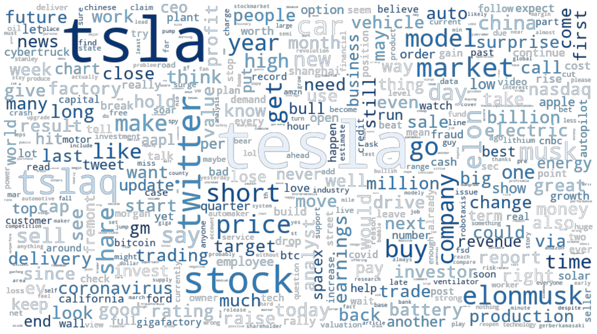
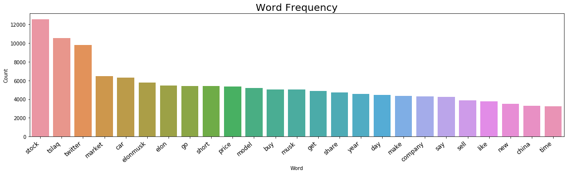
C. Word Cloud and Frequency Analysis
After cleaning, tokenizing and lemmatizing our data, we wanted to see when people mentioned our stocks on Twitter, what are the most frequently mentioned words. We did a frequency analysis of our tweet-word-list and formed WordCloud, the word-frequency plot and also the dataframe of the most frequent words people mentioned. We eliminated the single letters, special characters and invalid words such as “inc”, “com” and “pic” from the list to keep the word lists more relevant.
|
|
|
|
|
|
In order to illustrate what we did, I showed the full analysis process of the stock TSLA. Following are the WordCloud of the tesla tweets, word frequency plot.
|
|
For the readability of this paper, we hid the WordCloud and the plots for the rest 9 stocks, however, we summarized the most frequently used words for the 10 stocks in our portfolio in the following dataframe.
|
|
| id | tesla | netflix | microsoft | zoom | apple | amazon | sony | nvidia | ||
|---|---|---|---|---|---|---|---|---|---|---|
| 0 | stock | stock | corp | video | stock | nan | stock | goog | stock | |
| 1 | tslaq | stock | stock | market | check | jack | alphabet | aapl | amd | |
| 2 | earnings | market | security | price | stock | fb | stock | apple | earnings | |
| 3 | market | price | rating | verb | iphone | price | cloud | playstation | price | |
| 4 | car | dis | communication | market | like | nikkei | corporation | |||
| 5 | elonmusk | new | change | new | buy | tweet | apple | tokyo | target | |
| 6 | elon | high | result | msft | buy | company | go | coronavirus | jpm | |
| 7 | go | buy | surprise | use | coronavirus | aapl | get | aapl | msft | high |
| 8 | short | stream | cloud | company | close | apple | trump | amzn | market | buy |
| 9 | price | market | team | conferencing | rating | earnings | user | new | rkuny | new |
| 10 | model | amzn | amzn | secure | earnings | get | company | fb | amzn | ai |
| 11 | buy | disney | apple | buy | china | fb | company | nflx | corp | |
| 12 | musk | subscriber | new | platform | change | say | time | amazon | goog | indicator |
| 13 | get | share | buy | tech | store | year | share | msft | get | share |
| 14 | share | watch | aapl | orcl | amzn | msft | would | rakuten | nasdaq | |
| 15 | year | trade | amazon | work | result | new | close | microsoft | pt | raise |
| 16 | day | long | work | co | year | time | say | say | stock | short |
| 17 | make | short | earnings | launch | share | black | make | make | therealthing | market |
| 18 | company | content | company | crm | msft | bezos | ceo | work | theoneandonly | analyst |
| 19 | say | see | say | user | say | share | buy | business | fb | trade |
| 20 | sell | close | price | market | company | high | day | year | sensor | close |
| 21 | like | amazon | year | shop | surprise | one | new | ad | bac | data |
| 22 | new | year | coronavirus | go | sell | wireless | see | revenue | year | center |
| 23 | china | go | corporation | people | nasdaq | microsoft | year | youtube | buy | rating |
| 24 | time | target | report | partner | amazon | day | account | covid | game | report |
5. Trading Strategy
Warren Buffet once said, We simply attempt to be fearful when others are greedy and to be greedy only when others are fearful. His words are the source of our idea of this strategy.
Our strategy is based on people’s reaction of today’s market. We collected every tweet from today’s 16:00(today’s market close) to next day’s 9:00 (next day’s market open). Based on people’s attitude towards today’s market performance, we make the opposite move.
A. Original Plan
Go long three stocks which have the lowest score and short three stocks with have the highest score.
|
|
| time | tesla | netflix | microsoft | zoom | apple | amazon | sony | nvidia | ||
|---|---|---|---|---|---|---|---|---|---|---|
| 2020-01-03 | 0.333333 | 0.333333 | 0.000000 | -0.333333 | 0.333333 | 0.000000 | -0.333333 | 0.000000 | -0.333333 | 0.000000 |
| 2020-01-06 | 0.333333 | 0.000000 | 0.000000 | -0.333333 | 0.333333 | 0.333333 | 0.000000 | 0.000000 | -0.333333 | -0.333333 |
| 2020-01-07 | 0.333333 | 0.333333 | -0.333333 | -0.333333 | 0.333333 | 0.000000 | 0.000000 | 0.000000 | 0.000000 | -0.333333 |
| 2020-01-08 | 0.333333 | 0.000000 | 0.000000 | -0.333333 | 0.333333 | 0.000000 | 0.333333 | 0.000000 | -0.333333 | -0.333333 |
| 2020-01-09 | 0.333333 | 0.000000 | 0.333333 | -0.333333 | 0.333333 | -0.333333 | 0.000000 | 0.000000 | 0.000000 | -0.333333 |
| … | … | … | … | … | … | … | … | … | … | … |
| 2020-05-22 | 0.333333 | 0.333333 | 0.000000 | -0.333333 | 0.000000 | 0.000000 | 0.000000 | -0.333333 | -0.333333 | 0.333333 |
| 2020-05-26 | 0.000000 | 0.000000 | 0.000000 | -0.333333 | 0.333333 | -0.333333 | 0.333333 | -0.333333 | 0.000000 | 0.333333 |
| 2020-05-27 | 0.333333 | 0.000000 | -0.333333 | 0.000000 | 0.333333 | 0.000000 | 0.333333 | 0.000000 | -0.333333 | -0.333333 |
| 2020-05-28 | 0.333333 | 0.000000 | -0.333333 | 0.000000 | 0.333333 | -0.333333 | 0.333333 | 0.000000 | 0.000000 | -0.333333 |
| 2020-05-29 | 0.333333 | 0.000000 | -0.333333 | 0.000000 | 0.333333 | -0.333333 | 0.333333 | 0.000000 | -0.333333 | 0.000000 |
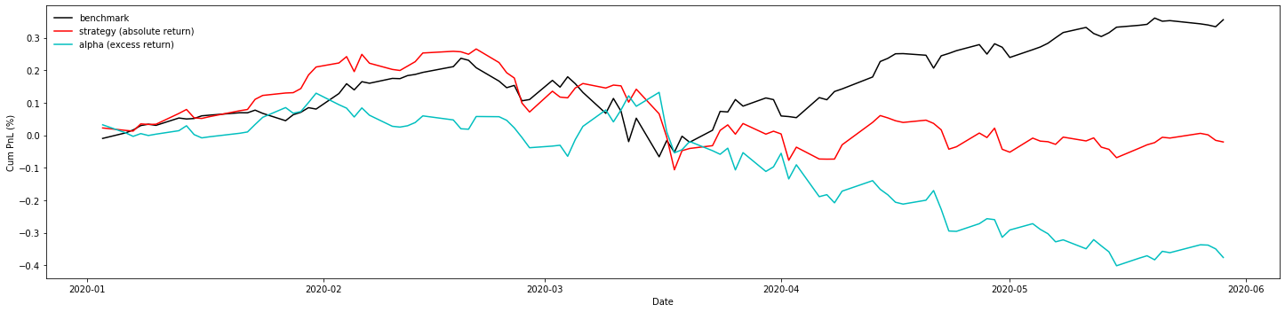
We set the benchmark of this strategy to be hold the 10 stocks evenly everyday. Also, we set the alpha to be the excess return of the strategy.
|
|
|
|
SR(benchmark) = 1.87
SR(strategy) = -0.10
SR(alpha) = -1.78

Sortino(benchmark) = 2.45
Sortino(strategy) = -0.13
Sortino(alpha) = -2.33

Max_Drawdown(benchmark) = 27.9%
Max_Drawdown(strategy) = 32.5%
Max_Drawdown(alpha) = 44.1%
From the result, we could see that the Sharpe Ratio of our strategy is not good…(negative SR), so we tried to improve our strategy.
B. Improvement
Instead of taking the highest three scores and lowest three scores, we took the sum of every tweet’s positive sentiment score and also negative sentiment scores in this time period (which indicates people’s attitudes towards today’s market performance by sentiment score and also the volume, the higher the volume, the more satisfied/disappointed people are). Based on the sum of the score we got for each stock, we normalize our positive and negative scores by seperately dividing the positive/negative sums of the sentiment scores to achieve market neutral, which means this does not cost us but in the meantime makes us money.
|
|
| time | tesla | netflix | microsoft | zoom | apple | amazon | sony | nvidia | ||
|---|---|---|---|---|---|---|---|---|---|---|
| 2020-01-03 | 0.401892 | 0.114972 | 0.059096 | -0.000000 | 0.330018 | 0.020177 | 0.009599 | 0.044186 | 0.008309 | 0.011751 |
| 2020-01-06 | 0.270341 | 0.065981 | 0.042288 | -0.000000 | 0.393034 | 0.095976 | 0.058378 | 0.040528 | 0.020787 | 0.012688 |
| 2020-01-07 | 0.442299 | 0.105930 | 0.021281 | -0.000000 | 0.201535 | 0.080591 | 0.065456 | 0.041283 | 0.026490 | 0.015135 |
| 2020-01-08 | 0.407693 | 0.066788 | 0.079381 | 0.009896 | 0.220641 | 0.052692 | 0.103467 | 0.031961 | 0.003662 | 0.023819 |
| 2020-01-09 | 0.360541 | 0.041014 | 0.081616 | 0.000709 | 0.361786 | 0.014596 | 0.078035 | 0.021689 | 0.024410 | 0.015605 |
| … | … | … | … | … | … | … | … | … | … | … |
| 2020-05-22 | 0.209791 | 0.150681 | 0.040223 | 0.017995 | 0.136417 | 0.125920 | 0.106557 | 0.020171 | 0.032025 | 0.160221 |
| 2020-05-26 | 0.144673 | 0.100749 | 0.102627 | 0.014581 | 0.261007 | 1.000000 | 0.154036 | 0.018609 | 0.032293 | 0.171425 |
| 2020-05-27 | 0.279436 | 0.054341 | 0.014196 | 0.023837 | 0.138186 | 0.071761 | 0.367798 | 0.029868 | 0.000406 | 0.020169 |
| 2020-05-28 | 0.096364 | 0.065429 | 0.617590 | 0.011994 | 0.216065 | 0.382410 | 0.526869 | 0.055728 | 0.019243 | 0.008308 |
| 2020-05-29 | 0.235185 | 0.031032 | 0.331849 | 0.029525 | 0.125487 | 0.668151 | 0.526221 | 0.032061 | -0.000000 | 0.020488 |
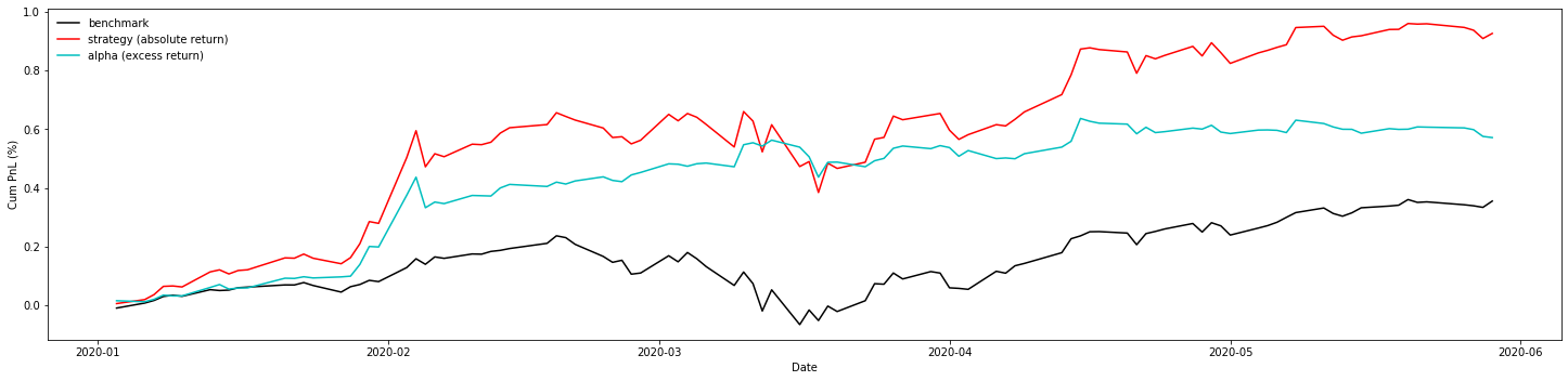
To evaluate the performance, like before, we also set the benchmark of this strategy to be hold the 10 stocks evenly everyday. Also, we set the alpha to be the excess return of the strategy.
|
|
|
|
SR(benchmark) = 1.87
SR(strategy) = 2.94
SR(alpha) = 3.01

Sortino(benchmark) = 2.45
Sortino(strategy) = 4.36
Sortino(alpha) = 5.03

Max_Drawdown(benchmark) = 27.9%
Max_Drawdown(strategy) = 27.1%
Max_Drawdown(alpha) = 12.2%
From the Sharpe ratio and the result we got, there’s a huge improvement. It illustrates that insteading of choosing the best and worse to go long and short evenly, we normally distribute our positions based on their level of scores. It’s more statistically significant. This is the strategy we’re gonna use.
C. Monthly Analysis
After setting the strategy, we digged into the monthly ratio to see the monthly performance.
|
|
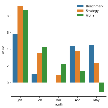
a. Sharpe Ratio
|
|
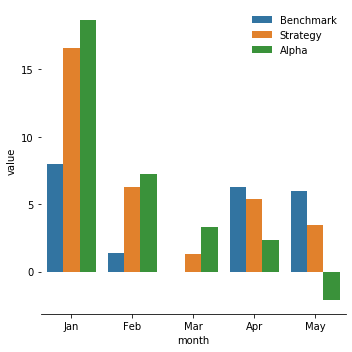
b. Sortino Ratio
|
|
|
|
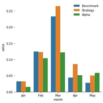
From the PNL plot we drew in the last section, we could see the performance of the strategy tends to be less effective in April and May. After plotting the three ratios of our monthly data, it’s obvious that our alpha and strategy’s edges are dimming from April to May (Sharpe Ratio and Sortino Ratio are dropping significantly and the maximum drawdown is increasing). On the contrary, the performance of the benchmark(hold ten stocks evenly every day) is steady and decent comparing with the other two. So, if we want to better our strategy’s performance further, we could use the benchmark strategy and just buy and hold equal position of ten stocks in April and May. Combining with what happened in the states( COVID-19, quarantine, Trump’s false administration…), we concluded that our strategy gradually lost its edge during this period because people’s attitudes and judgements of market are not only based on the performance of the stocks and their rational analysis, but also on their emotions(especially rage). In this case, the sentiment analysis is not effective like before. It shows the limitation of our strategy: people are emotional creatures when unusual things happen, so investing based on people’s attitudes towards market can be profitable but in the meantime risky.
6. Conclusion
Our strategy is based on NLP analysis towards twitters of the stock markets. The performance of our strategy shows the significance of the signal; however, during special time period, this strategy could be less effective and more volatile. In order to better improve the strategy’s performance, we could enlarge our portfolio pool, which would definitely increase the accuracy of the signal. Also, expanding the backtest period would also be effective.
Reference
Clarence C.Y. Kwan (1998). “A note on market-neutral portfolio selection”. Journal of BANKING & FINANCE.
Tushar Rao and Saket Srivastava(2013).“Analyzing Stock Market Movements Using Twitter Sentiment Analysis”. LINCOLN REPOSITORY.
Yuexin Mao, Bing Wang, Wei Wei, Benyuan Liu. “Correlating S&P 500 Stocks with Twitter Data”. ACM Digital Library.
Anshul Mittal and Arpit Goel(2011). “Stock Prediction Using Twitter Sentiment Analysis”.