Spread Trading Strategy

This is a spreading strategy which is based on M-day returns of two highly related futures. The idea of this strategy is to hedge the risk of buying and holding one specific future with increasing returns by holding the opposite position of another future.

We define g and j be our trading thresholds in this strategy. Besides, we also have stop-loss threshold s. Our initial capital K is $100MM.

1. Introduction

In this section we give brief intro on the strategy we’re about to implement.

The rule of spread strategy

After confirming our pair of futures, when market opnes, we enter the market and observe our current position:

• If we’re currently not trading: we observe our strategy spread, if the -g < r < g, we do nothing today; if r > g, we go short our spread today; if r < g, we go long our spread.

• If we’re currently longing in spread: we ovserve our strategy spread, if r < -j, we do nothing today; if r > g, we go short our spread today; if -j < r < g, we close our position.

• If we’re currently going short in spread: we ovserve our strategy spread, if r > j, we do nothing today; if r < -g, we go short our spread today; if -g < r < j, we close our position.

Besides the observation of our spread and thresholds, we also should keep an eye on the stop-loss threshold. If the strategy losts certain percentage of our capital, the stop-loss shreshold will be triggered and our positoin will be closed for the rest of the month.

What’s more, every last day of each month, our position will be closed once.

2. Data Preparation

Introduction of the packages in spread trading

We’re using several really important python pac

• Pandas: dataframe manipulation
• NumPy: support for mathematical functions and computation of arrays and matrics
• Statsmodel: statistical analysis
• Matplotlib: plot tools
• Seaborn: statistical data visualization
• Scipy: statistical analysis
• tqdm: progress bar
• itertools: produce grid of parameters

 1
 2
 3
 4
 5
 6
 7
 8
 9
10
11
12
13

import quandl
import pandas as pd
import numpy as np
import warnings
import statsmodels.api as sm
import statsmodels.formula.api as smf
import matplotlib.pyplot as plt
import seaborn as sns
from tqdm.auto import tqdm
from scipy import stats
from itertools import product
from statsmodels.tsa.stattools import adfuller
from statsmodels.graphics.tsaplots import plot_acf

1
2
3
4
5

warnings.filterwarnings('ignore')
pd.set_option('max_rows', 100)
plt.rcParams['figure.figsize'] = (10, 4)

quandl.ApiConfig.api_key = 'yFs2mPKxvfCC26C4vG3K'

Obtaining data from Quandl

From Quandl’s OWF ( OptionWorks Futures Options ) database, we obtain data of our future pair: ICE_T_T ( ICE WTI Crude Oil T Futures Options Implied Volatility Model ) and ICE_G_G ( ICE WTI Gas Oil Futures Options Implied Volatility Model ) from 2017-12-02 to 2019-08-31.

For this strategy, we use the second month futures prices to define our future prices. The definition of second month is the contract where the number of days to futures expiration is the smallest available value greater than 30.

speck gas oil：metre tonne crude oil：barrel 7.45

Relationship between the spread pair (WTI Crude Oil and Gas Oil) (ICE_T_T and ICE_G_G)

We now look at the relationship between crede oil and gas oil in the real world. Here’s the relationship between those two:

From the picture, we could see that both light gas oil and heavy gas oil are the product of the crude distillation, which means they’re high correlated with each other. Gas oil price is higher than crude oil since during the process of production, it adds refinement value to the gas oil. That’s why their difference are relatively the same as the time changes.

One thing which is also worth meantioning is that the unit of Crude Futures is barrel, and the trading unite of the Gas Oil Futures is metric tonne. By researching, I found out that 1 metric tonne is relatively 7.45 barrels. That’s why during our calculation of spread, we need the multiplier 1/7.45 below.

 1
 2
 3
 4
 5
 6
 7
 8
 9
10
11
12
13
14
15
16
17
18
19
20
21
22
23
24
25
26
27
28
29
30
31
32
33
34
35
36
37
38
39
40
41
42
43
44

sdate = '2017-12-02'
edate = '2019-08-31'

cache = {}

month = ['H', 'M', 'U', 'Z']
year = ['2018', '2019']
list_of_X = []
list_of_Y = []

def get(symbol):
    if symbol not in cache: cache[symbol] = quandl.get(symbol, start_date=sdate, end_date='2020-04-01')
    return cache[symbol]

for n in year:
    for m in month:
        futureX = get(f'OWF/ICE_T_T_{m}{n}_IVM')
        futureY = get(f'OWF/ICE_G_G_{m}{n}_IVM')
        futureX = futureX[futureX['DtT'] > 30]
        futureY = futureY[futureY['DtT'] > 30]
        list_of_X.append(futureX)
        list_of_Y.append(futureY)

X_price = dict()
Y_price = dict()
multiplier = 1 / 7.45

for date in pd.bdate_range(sdate, edate):
    list_of_X_available = [X for X in list_of_X if date in X.index]
    if list_of_X_available:
        price = min(list_of_X_available, key=lambda df: df.loc[date, 'DtT']).loc[date, 'Future']
        X_price[date] = price
        
for date in pd.bdate_range(sdate, edate):
    list_of_Y_available = [Y for Y in list_of_Y if date in Y.index]
    if list_of_Y_available:
        price = min(list_of_Y_available, key=lambda df: df.loc[date, 'DtT']).loc[date, 'Future']
        Y_price[date] = price
        
X_price = pd.Series(X_price)
Y_price = pd.Series(Y_price)
rt = multiplier * Y_price - X_price
X_pnl = X_price.diff()
Y_pnl = Y_price.diff()

3. Strategy and Backtest

Several data we use here:

• X_price: the price of Crude Oil Futures
• Y_price: the price of Gas Oil Futures

After getting the data we need, we do several computations:

• Raw Spread (rt): multiplier * Y_price - X_price
• Moving Average (MA): moving average of raw spread
• Stretegy spread (st): rt - MA

1
2
3
4

data = pd.DataFrame(rt, columns=['Raw spread'])
M = 20
data['MA'] = data['Raw spread'].rolling(M, min_periods=1).mean()
data['Strategy Spread'] = data['Raw spread'] - data['MA']

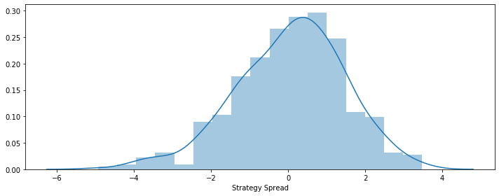
Firstly, we could plot the distribution (histogram) of the spread.

1
2
3

sns.distplot(data['Strategy Spread'])
plt.tight_layout()
plt.show()

Also, we could plot the fitted normal distribution and t-distribution in order to compare.

 1
 2
 3
 4
 5
 6
 7
 8
 9
10
11
12
13
14
15
16
17
18
19

fig = plt.figure()

ax = fig.add_subplot(111)
ax.hist(data['Strategy Spread'], bins=40, density=True)
x_grid = np.linspace(-6, 6, 1200)

params1 = stats.norm.fit(data['Strategy Spread'])
fit_pdf1 = stats.norm.pdf(x_grid, *params1)
plt.plot(x_grid, fit_pdf1, label='Normal')

params2 = stats.t.fit(data['Strategy Spread'])
fit_pdf2 = stats.t.pdf(x_grid, *params2)
plt.plot(x_grid, fit_pdf2, label="t")

ax.set_xlabel("Strategy Spread")
ax.set_ylabel("density")

plt.tight_layout()
plt.show()

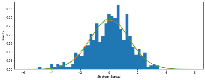
From the histrogram of the strategy spread, we could see that normal and t distribution both fit the distribution pretty well, which implies that it is normal distributed.

Stationarity test

In order to do the spread trading, we assume the pair’s spread is stational. Before actually testing the strategy and tuning the parameter, we firstly check the stionarity of the spread by doing the Ad-Fuller test.

We do the Unit-Root test, so our null hypothesis is that the strategy spread only has one unit root.

1
2

ad_result = adfuller(data['Strategy Spread'])
ad_result

(-5.36982767996684,
 3.918169723518303e-06,
 13,
 435,
 {'1%': -3.4454725477848998,
  '5%': -2.8682072297316794,
  '10%': -2.570321396485665},
 1052.6004685638443)

Since the p-value in the test is 3.918169723518303e-06, which is far less than 0.05, so we could reject the null hypothesis and draw the conclusion that the spread has stationarity and we could use the pair to do spread trading.

Backtest

Backtest is where we use the historical data to test our strategy. The logic of the backtest is the rule of the spread strategy I mentioned at the beginning of this notebook. Here, I wrote a function Backtest with the parameter S, M, g and j, which are the thresholds of our spread strategy. The Backtest returns the strategy’s daily pnl series with certain parameters we set at the beginning of the function.

For details of the backtest, I make comments of every crutial step.

 1
 2
 3
 4
 5
 6
 7
 8
 9
10
11
12
13
14
15
16
17
18
19
20
21
22
23
24
25
26
27
28
29
30
31
32
33
34
35
36
37
38
39
40
41
42
43
44
45
46
47
48
49
50
51
52
53
54
55
56
57
58
59
60
61
62
63
64

def backtest(S, M, g, j):
    st = rt - rt.rolling(M, min_periods=1).mean()  # strategy spread
    
    daily_pnl_series = []  # list of daily PNL
    total_value = 1e6  # initial capital
    x_pos = y_pos = tmr_pos = 0  # set initial spread position to 0 
    prev_day = -1  # the day before "today" 
    stoploss = False  # indicator: true if currently we're end of every month or we need to stop in order to stop the loss
    first_day = st.index[0]  # the first trading day
    
    for date in st.index:
        tdy_pos = tmr_pos  # every round of for loop, set today's opening position equal to yesterday's closing position
        
        if date.day < prev_day:
            tdy_pos = 0  # if it's first day of the month, then no position
            stoploss = False  # reset stoploss status on the first day of the month
        if stoploss:
            tdy_pos = 0  # if it's during stop loss period, then no position
        
        prev_day = date.day  # reset prev_day to be today's date
        
        if date != first_day:
            tdy_x_pnl = X_pnl[date]  # today's X's PNL
            tdy_y_pnl = Y_pnl[date]  # today's Y's PNL
            daily_pnl = tdy_x_pnl * x_pos + tdy_y_pnl * y_pos  # today's PNL 
        else:
            daily_pnl = 0
        daily_pnl_series.append(daily_pnl)  # append today's PNL into the list of daily PNL
        total_value += daily_pnl  # update total capital every day 

        if tdy_pos == 0:
            if st[date] > g:
                tmr_pos = -1
            elif st[date] < -g:
                tmr_pos = 1
            elif st[date] > -g and st[date] < g:
                pass
    
        elif tdy_pos == 1:
            if st[date] > g:
                tmr_pos = -1
            elif st[date] < -j:
                pass
            elif st[date] > -j and st[date] < g:
                tmr_pos = 0
                
        elif tdy_pos == -1:
            if st[date] > j:
                pass
            elif st[date] < -g:
                tmr_pos = 1
            elif st[date] > -g and st[date] < j:
                tmr_pos = 0
        
        if tdy_pos == 0 and tmr_pos != 0:  # update X position and Y position if we start a new trading
            x_pos = -round(total_value / 2 / X_price[date]) * tmr_pos
            y_pos = round(total_value / 2 / Y_price[date]) * tmr_pos
            
        if date != first_day: 
            if daily_pnl < -S * total_value:
                stoploss = True  # to determine when to start a stoploss
    
    daily_pnl_series = pd.Series(daily_pnl_series, index=st.index)
    return daily_pnl_series

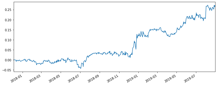
Here, I choose a set of thresholds (S=0.01, M=5, g=0.5, j=0.4) in order to make illustrations. After getting the daily_pnl series of the strategy, we could easily draw the cumulative_pnl plot to show the strategy’s performance.

1
2
3
4
5

daily_pnl = backtest(0.01, 5, .5, .4)
cum_pnl = daily_pnl.cumsum() / 1e6
cum_pnl.plot()
plt.tight_layout()
plt.show()

Parameter Tuning

Clearly, choosing thresholds by hands is not working here. It’s not efficient. More importantly, it’s not gonna help us find the best strategy. That’s why we should do the parameter tuning here. Before getting into that, I also want to use four indexes to judge if the strategy is good enough.

They are:

• Sharpe Ratio: return of an investment compared to its risk
• Sortino Ratio: risk-adjusted return of a strategy
• Maximnm Drawdown: maximum observed loss from a peak to a trough
• Winning Rate: the percentage of winning

Create Sharpe Ratio function.

1

sharpe = lambda x: x.mean() / x.std() * 252**.5

Create Sortino Ratio function.

1

sortino = lambda x: x.mean() / (((x - x.mean())**2 * (x < 0)).mean())**.5 * 252**.5

Create Maximum Drawdown function.

1
2
3

def maximum_drawdown(x, initial_value=1e6):
    v = x.cumsum() + initial_value
    return (1 - v / v.cummax()).max()

Create Winning Rate function.

1

win_rate = lambda x: (x > 0).mean()

Set parameter grids.

Since there’re only four parameters in our paremeter tuning, I choose to use a simple for-loop ( actually there’re four layers of calculations here ) instead of machine learning method. The advantage of this method is that by setting one index ( I use Sharpe Ratio here to be the index ), it is efficient to compute. However, there’re also disadvantages of this method. We could not look at the four indexes at the same time.

 1
 2
 3
 4
 5
 6
 7
 8
 9
10
11
12
13
14
15
16

S_grid = np.arange(0.01, 0.11, 0.1)
M_grid = [5, 10, 15, 20]
g_grid = np.arange(0.1, 3.1, 0.1)
j_grid = np.arange(-2, 2.1, 0.1)
params_grid = list(product(S_grid, M_grid, g_grid, j_grid))

max_sharpe = -float('inf')

for params in tqdm(params_grid):
    daily_pnl = backtest(*params)
    sharpe_ratio = sharpe(daily_pnl)
    if sharpe_ratio > max_sharpe:
        max_sharpe = sharpe_ratio
        best_params = params

print('The best params are S = {:.2f}, M = {:.0f}, g = {:.1f} and j = {:.1f} with the best Sharpe Ratio {:.2f}.'.format(*best_params, max_sharpe))

The best params are S = 0.01, M = 20, g = 3.0000000000000004 and j = 2.0000000000000036 with the best Sharpe Ratio 2.503240431597306.

After the parameting tuning, we could compute the four functions seperately to see the performance of this set of thresholds. From the result, we could see that the Sharpe Ratio of this strategy is 2.5, which is pretty high here.

1

print([func(backtest(*best_params)) for func in [sharpe, sortino, maximum_drawdown, win_rate]])

[2.503240431597306, 3.99927975276015, 0.046804254666939826, 0.5412026726057907]

To see if the parameter tuning actually works, I also compute the four indexes of the previous set of thresholds I randomly picked. From the result, we could see that although we only use the Sharpe Ratio to optimize the performance of our strategy, all of my four indexes improved, which means although there’re limitations of the parameter tuning, it’s still a solid overall improvement of my strategy.

1

print([func(backtest(0.01, 5, .5, .4)) for func in [sharpe, sortino, maximum_drawdown, win_rate]])

[1.218223449118886, 1.8641248661345056, 0.0533043738617216, 0.5100222717149221]

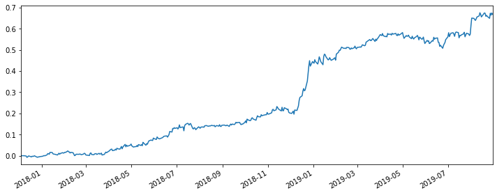
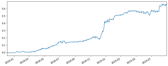
Like before, I also draw the cumulative return plot of the optimized strategy here. From the strategy, we could tell the optimization is pretty solid. The overall return in the end of the time period we choose is almost 70%. What’s more, the performance is more stable and less volatile, which is good for traders and investors.

1
2
3
4

best_cum = backtest(*best_params).cumsum() / 1e6
best_cum.plot()
plt.tight_layout()
plt.show()

4. Regression Analysis

After the spread strategy, we could also combine our spread strategy with the Fama-French factor(s). By holding the opposite position of Fama-French foctor(s), we hedge the risk of the spread strategy itself.

About the Fama-French model factors, there’re three factors:

• Small Minus Big (SMB): “size effect”, small companies overperform larger ones over the long-term
• High Minus Low (HML): outperformance of value stocks over growth stocks
• Excess Return (Mkt-Rf): excess return of the market

By using Ordinary Least Squares regression, we hedge the risk of our spread strategy by holding opposite positions of SMB/HML/Mkt-Rf or the three Fama-French factors together. The residual of our regression will be the daily pnl series of the strategy. By analyzing that, we could see the performance and determine if the hegde works.

Obtain data of daily Fama-French factor returns

We obtain the daily Fama-French factor returns from Ken French’s website.

1
2
3
4
5
6
7

ff_factors = pd.read_csv('../HW2/F-F_Research_Data_Factors_daily.CSV', header=3, index_col=0)
ff_factors = ff_factors.iloc[:-1]
ff_factors.index = pd.to_datetime(ff_factors.index)
ff_factors = ff_factors[sdate:edate]
ff_factors['PNL'] = backtest(*best_params)
ff_factors.columns = ['Mkt_RF', 'SMB', 'HML', 'RF', 'PNL']
ff_factors

Regression between daily_pnl of the spread strategy and fama-french factor “SMB”

1
2

model_smb = smf.ols('PNL ~ SMB + 0', data=ff_factors).fit()
print(model_smb.summary())

                                 OLS Regression Results                                
=======================================================================================
Dep. Variable:                    PNL   R-squared (uncentered):                   0.008
Model:                            OLS   Adj. R-squared (uncentered):              0.006
Method:                 Least Squares   F-statistic:                              3.507
Date:                Wed, 22 Apr 2020   Prob (F-statistic):                      0.0618
Time:                        21:47:45   Log-Likelihood:                         -4636.0
No. Observations:                 438   AIC:                                      9274.
Df Residuals:                     437   BIC:                                      9278.
Df Model:                           1                                                  
Covariance Type:            nonrobust                                                  
==============================================================================
                 coef    std err          t      P>|t|      [0.025      0.975]
------------------------------------------------------------------------------
SMB        -1680.5135    897.342     -1.873      0.062   -3444.155      83.128
==============================================================================
Omnibus:                      169.503   Durbin-Watson:                   1.950
Prob(Omnibus):                  0.000   Jarque-Bera (JB):             1364.249
Skew:                           1.441   Prob(JB):                    5.71e-297
Kurtosis:                      11.152   Cond. No.                         1.00
==============================================================================

Warnings:
[1] Standard Errors assume that the covariance matrix of the errors is correctly specified.

1
2
3
4

cum_smb = model_smb.resid.cumsum() / 1e6
cum_smb.plot()
plt.tight_layout()
plt.show()

1

print([func(model_smb.resid) for func in [sharpe, sortino, maximum_drawdown, win_rate]])

[2.505257399243229, 4.025154172157131, 0.04379745877202246, 0.5616438356164384]

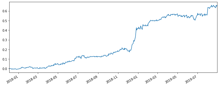
From the cumulative return plot and the four indexes we could see that, although the performance of this hedge is good, comparing with the spread strategy itself, it does not become better, which means the hedge does not optimize the strategy.

From my perspective, I think the reason why this hedge may be a good strategy is that SMB represents the idiosyncratic risks of individual companies in the market. By doing this hedge, we’re actually hedging out these risk factors.

Regression between daily_pnl of the spread strategy and fama-french factor “HML”

1
2

model_hml = smf.ols('PNL ~ HML + 0', data=ff_factors).fit()
print(model_hml.summary())

                                 OLS Regression Results                                
=======================================================================================
Dep. Variable:                    PNL   R-squared (uncentered):                   0.002
Model:                            OLS   Adj. R-squared (uncentered):             -0.000
Method:                 Least Squares   F-statistic:                             0.8283
Date:                Wed, 22 Apr 2020   Prob (F-statistic):                       0.363
Time:                        21:39:23   Log-Likelihood:                         -4637.3
No. Observations:                 438   AIC:                                      9277.
Df Residuals:                     437   BIC:                                      9281.
Df Model:                           1                                                  
Covariance Type:            nonrobust                                                  
==============================================================================
                 coef    std err          t      P>|t|      [0.025      0.975]
------------------------------------------------------------------------------
HML         -735.0567    807.672     -0.910      0.363   -2322.462     852.349
==============================================================================
Omnibus:                      160.188   Durbin-Watson:                   1.965
Prob(Omnibus):                  0.000   Jarque-Bera (JB):             1194.160
Skew:                           1.369   Prob(JB):                    4.92e-260
Kurtosis:                      10.612   Cond. No.                         1.00
==============================================================================

Warnings:
[1] Standard Errors assume that the covariance matrix of the errors is correctly specified.

1
2
3
4

cum_hml = model_hml.resid.cumsum() / 1e6
cum_hml.plot()
plt.tight_layout()
plt.show()

1

print([func(model_hml.resid) for func in [sharpe, sortino, maximum_drawdown, win_rate]])

[2.490594369232336, 3.9826647643042516, 0.04296930198567317, 0.5388127853881278]

Same conlusion as the regression of SMB, although it’s a good strategy, it did not outperform the original spread strategy in terms of the cumulative return and the four indexes.

Regression between daily_pnl of the spread strategy and fama-french factor “Mkt-RF”

1
2

model_mkt = smf.ols('PNL ~ Mkt_RF + 0', data=ff_factors).fit()
print(model_mkt.summary())

                                 OLS Regression Results                                
=======================================================================================
Dep. Variable:                    PNL   R-squared (uncentered):                   0.037
Model:                            OLS   Adj. R-squared (uncentered):              0.035
Method:                 Least Squares   F-statistic:                              16.71
Date:                Wed, 22 Apr 2020   Prob (F-statistic):                    5.17e-05
Time:                        21:36:27   Log-Likelihood:                         -4545.0
No. Observations:                 438   AIC:                                      9092.
Df Residuals:                     437   BIC:                                      9096.
Df Model:                           1                                                  
Covariance Type:            nonrobust                                                  
==============================================================================
                 coef    std err          t      P>|t|      [0.025      0.975]
------------------------------------------------------------------------------
Mkt_RF     -1516.4122    370.913     -4.088      0.000   -2245.408    -787.416
==============================================================================
Omnibus:                       59.934   Durbin-Watson:                   2.670
Prob(Omnibus):                  0.000   Jarque-Bera (JB):              400.301
Skew:                          -0.316   Prob(JB):                     1.19e-87
Kurtosis:                       7.641   Cond. No.                         1.00
==============================================================================

Warnings:
[1] Standard Errors assume that the covariance matrix of the errors is correctly specified.

1
2
3
4

cum_mkt = model_mkt.resid.cumsum() / 1e6
cum_mkt.plot()
plt.tight_layout()
plt.show()

1

print([func(model_mkt.resid) for func in [sharpe, sortino, maximum_drawdown, win_rate]])

[0.3184069744735868, 0.4461720053872383, 0.10328493002974315, 0.5068493150684932]

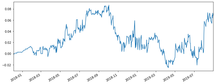
Unlike the previous two regressions we did, this hedge does not do well. The return is pretty low and the four indexes are also not impressive at all.

From my personal understanding, I‘m thiking maybe the reason is the crude oil and the gas oil (energy market) is so correlated with the market return that the spread between them are relatively small, which makes this kind of hedge’s return not significant.

Regression between daily_pnl of the spread strategy and the three fama-french factors

1
2

model_ff = smf.ols('PNL ~ SMB + HML + Mkt_RF + 0', data=ff_factors).fit()
print(model_ff.summary())

                                 OLS Regression Results                                
=======================================================================================
Dep. Variable:                    PNL   R-squared (uncentered):                   0.011
Model:                            OLS   Adj. R-squared (uncentered):              0.005
Method:                 Least Squares   F-statistic:                              1.668
Date:                Wed, 22 Apr 2020   Prob (F-statistic):                       0.173
Time:                        21:49:20   Log-Likelihood:                         -4635.2
No. Observations:                 438   AIC:                                      9276.
Df Residuals:                     435   BIC:                                      9289.
Df Model:                           3                                                  
Covariance Type:            nonrobust                                                  
==============================================================================
                 coef    std err          t      P>|t|      [0.025      0.975]
------------------------------------------------------------------------------
SMB        -1856.8941    910.402     -2.040      0.042   -3646.228     -67.560
HML        -1001.3976    849.643     -1.179      0.239   -2671.313     668.518
Mkt_RF        -3.8589    477.602     -0.008      0.994    -942.554     934.837
==============================================================================
Omnibus:                      161.307   Durbin-Watson:                   1.950
Prob(Omnibus):                  0.000   Jarque-Bera (JB):             1200.859
Skew:                           1.381   Prob(JB):                    1.73e-261
Kurtosis:                      10.627   Cond. No.                         2.12
==============================================================================

Warnings:
[1] Standard Errors assume that the covariance matrix of the errors is correctly specified.

1
2
3
4

cum_ff = model_ff.resid.cumsum() / 1e6
cum_ff.plot()
plt.tight_layout()
plt.show()

1

print([func(model_ff.resid) for func in [sharpe, sortino, maximum_drawdown, win_rate]])

[2.4056098457815827, 3.855107672834527, 0.04787717023424776, 0.5593607305936074]

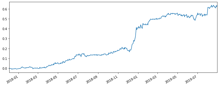
Like the SMB and HML, using the Fama-French factors to hedge is a decent strategy. However, like the previous two hedges, it does not outperform the optimized version of our spread strategy.

Comparison

By plotting all the five return curves together, we could find out that our optimized spread strategy’s performance after the paremeter tuning is the best.

1
2
3
4
5
6
7
8

(model_smb.resid.cumsum() / 1e6).plot(label='hedged-smb', c='r')
(model_ff.resid.cumsum() / 1e6).plot(label='hedged-ff', c='c')
(model_hml.resid.cumsum() / 1e6).plot(label='hedged-hml')
(model_mkt.resid.cumsum() / 1e6).plot(label='hedged-mkt')
(backtest(*best_params).cumsum() / 1e6).plot(label='unhedged', c='k')
plt.legend(frameon=False)
plt.tight_layout()
plt.show()

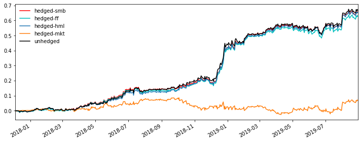
However…

Here’s one thing that some people may neglect about the regression/hedge that we did just now. We’re using the future information to compute the regression and do the backtest, which is forward-looking. In the real world, we could not do this on any day within this time period unless we’re looking back at the historical data. So even if the strategy is working and doing really well, we could not utilize it in the real world senario. A better alternative would be just use the in-sample data to do rolling regressions instead of one single large one for all.

5. Conclusion

In a nutshell, spread trading on commodity markets, especially in our case, in energy markets, is exceptionally profitable mainly in that the different energy products are inner related - most are products of the few resources and the value-adds are relatively fixed over time. The same logic should apply in many other products and markets and we’d be more than willing to dig into those.