Robust and Bayesian Regression Comparison

Robust techniques and variable selection can help us obtain more stable linear fits. In this post, I used return regressions against returns on State Street sctors ETFs to test this fact. By computing out-of-sample regression, I contrast the performance of OLS regression, robust regression(huber and tukey) and positive lasso regressions.

 1
 2
 3
 4
 5
 6
 7
 8
 9
10
11
12

import os
import quandl
import pickle
import warnings
import numpy as np
import pandas as pd
import seaborn as sns
from tqdm.auto import tqdm
import statsmodels.api as sm
from functools import lru_cache
import matplotlib.pyplot as plt
from sklearn import linear_model

1. Import EOD from Quandl

First we load ETF and stocks that satisfies our requirements. By requirement we are saying each of the following stocks

1. Has 41 days of adj close prices from 2019/01/01 to 2019/03/01 inclusive, and
2. Can give 1, 3 and 6 non-zero betas from Lasso (both with and without positive beta restriction) regression for later analysis.

The full list of tickers are as below:

1
2
3
4

ETFs = ['XLC', 'XLY', 'XLP', 'XLE', 'XLF', 'XLV', 'XLI', 'XLB', 'XLRE', 'XLK', 'XLU']
stocks = ['AADR', 'AAON', 'ACER', 'ACIW', 'ACLS', 'ACM', 'ACT', 'ACWF', 'ACWI', 'ACWX',
          'ADT', 'AFT', 'AFTY', 'AGD', 'AGO_P_B', 'AHT', 'AIEQ', 'AIG_WS', 'AIRR', 'ALKS',
          'ALL', 'ALXN', 'AMGN', 'AMN', 'AMNB', 'AMOT', 'ANDE', 'ANSS', 'AOA', 'AON']

Now we start actual loading.

 1
 2
 3
 4
 5
 6
 7
 8
 9
10
11
12
13
14
15
16
17
18
19
20
21

tickers = ETFs + stocks
ETFs = ['intercept'] + ETFs

start_date = '2019-01-01'
end_date = '2019-03-01'

def get_eod(tic):
    return quandl.get(f'EOD/{tic}', start_date=start_date, end_date=end_date).Adj_Close

if os.path.isfile('EOD.pkl'):
    with open('EOD.pkl', 'rb') as f:
        EOD = pickle.load(f)
else:
    EOD = {}
    for tic in tqdm(tickers):
        try:
            EOD[tic] = get_eod(tic)
        except Exception:
            print(f'skip {tic} as it\'s missing in EOD dataset')
    with open('EOD.pkl', 'wb') as f:
        pickle.dump(EOD, f)

Compute each ticker’s daily return and then seperate the return into in-sample (the first 20 days) and out-of-sample (the last 20 days) data.

1
2
3
4
5
6

df_EOD = pd.DataFrame(EOD)
df_return = df_EOD.pct_change()
df_return.dropna(inplace=True)
df_return['intercept'] = 1
df_insample = df_return.iloc[:20]
df_outsample = df_return.iloc[20:]

2. Regression

In this part we perform regressions one by one. For each regression, we first run in-sample fitting to get the optimal configs (if any) and the in-sample betas. Then using the in-sample optimal configs we run out-of-sample regression to get the same amount of coefficients to calculate the in-to-out beta L2 norm as our robustness metric.

A. OLS regression

First is OLS regression.

a. In-sample

No optimization is required in OLS.

1
2
3
4
5

ols_insample_beta_dict = {}
for stock in stocks:
    reg_ols = sm.OLS(df_insample[stock], df_insample[ETFs]).fit()
    beta_insample = reg_ols.params
    ols_insample_beta_dict[stock] = beta_insample

b. Out-of-sample

As there’s no optimization, we simply rerun the same regression against the out-of-sample dataset.

1
2
3
4
5

ols_outsample_beta_dict = {}
for stock in stocks:
    reg_ols = sm.OLS(df_outsample[stock], df_outsample[ETFs]).fit()
    beta_outsample = reg_ols.params
    ols_outsample_beta_dict[stock] = beta_outsample

c. L2 norm

The L2 norm is calculated and stored for later analysis.

1
2
3
4
5
6

ols_insample_beta_df = pd.DataFrame(ols_insample_beta_dict)
ols_outsample_beta_df = pd.DataFrame(ols_outsample_beta_dict)
ols_beta_diff = ols_insample_beta_df - ols_outsample_beta_df

ols_l2_norm = (ols_beta_diff**2).sum()**.5
ols_l2_norm

AADR        1.353710
AAON        5.330675
ACER        4.029213
ACIW        4.501306
ACLS        6.978846
ACM         1.882538
ACT         1.235258
ACWF        0.918673
ACWI        0.740807
ACWX        1.695779
ADT         5.984692
AFT         1.338696
AFTY        4.282447
AGD         2.287036
AGO_P_B     1.096079
AHT         8.060704
AIEQ        0.888335
AIG_WS     14.980616
AIRR        1.498807
ALKS        4.509373
ALL         2.427588
ALXN        4.066937
AMGN        3.331021
AMN        13.501120
AMNB        3.191322
AMOT        2.786852
ANDE        3.685212
ANSS        3.813627
AOA         0.673246
AON         3.456226
dtype: float64

B. Huber

In Huber regression we have a penalty term with parameter t. Therefore we have the ability to optimize this t for in-sample fitting.

a. In-sample

We use grid search to perform the optimization.

 1
 2
 3
 4
 5
 6
 7
 8
 9
10
11
12
13
14

huber_insample_beta_dict = {}
huber_t_best = {}
t_grid = np.arange(1, 5, .1)
for stock in stocks:
    mse_best = float('inf')
    for t in t_grid:
        reg_huber = sm.RLM(df_insample[stock], df_insample[ETFs], M=sm.robust.norms.HuberT(t=t)).fit()
        mse = ((df_insample[stock] - reg_huber.fittedvalues)**2).mean()**.5
        if mse < mse_best:
            mse_best = mse
            huber_t_best[stock] = t
    reg_huber = sm.RLM(df_insample[stock], df_insample[ETFs], M=sm.robust.norms.HuberT(t=huber_t_best[stock])).fit()
    beta_insample = reg_huber.params
    huber_insample_beta_dict[stock] = beta_insample

b. Out-of-sample

We use the optimal t we found to run out-of-sample regression.

1
2
3
4
5

huber_outsample_beta_dict = {}
for stock in stocks:
    reg_huber = sm.RLM(df_outsample[stock], df_outsample[ETFs], M=sm.robust.norms.HuberT(t=huber_t_best[stock])).fit()
    beta_outsample = reg_huber.params
    huber_outsample_beta_dict[stock] = beta_outsample

c. L2 norm

1
2
3
4
5

huber_insample_beta_df = pd.DataFrame(huber_insample_beta_dict)
huber_outsample_beta_df = pd.DataFrame(huber_outsample_beta_dict)
huber_beta_diff = huber_insample_beta_df - huber_outsample_beta_df
huber_l2_norm = (huber_beta_diff**2).sum()**.5
huber_l2_norm

AADR        1.390011
AAON        5.330675
ACER        4.029213
ACIW        4.520645
ACLS        6.978846
ACM         1.723419
ACT         1.177438
ACWF        0.914225
ACWI        0.740807
ACWX        1.716467
ADT         5.984692
AFT         1.338696
AFTY        3.177647
AGD         2.287036
AGO_P_B     0.926278
AHT         8.060704
AIEQ        0.847107
AIG_WS     14.980616
AIRR        1.498807
ALKS        5.871315
ALL         2.642671
ALXN        4.030956
AMGN        3.331021
AMN        13.499555
AMNB        3.274254
AMOT        2.786852
ANDE        3.685212
ANSS        3.833712
AOA         0.742647
AON         3.454299
dtype: float64

C. Tukey

In Tukey regression there is, similar to Huber reg, a parameter c which is integers.

a. In-sample

We run grid search on c to find its optima based on minimizing in-sample MSE of residuals.

 1
 2
 3
 4
 5
 6
 7
 8
 9
10
11
12
13
14

tukey_insample_beta_dict = {}
tukey_c_best = {}
c_grid = range(1, 50)
for stock in stocks:
    mse_best = float('inf')
    for c in c_grid:
        reg_tukey = sm.RLM(df_insample[stock], df_insample[ETFs], M=sm.robust.norms.TukeyBiweight(c=c)).fit()
        mse = ((df_insample[stock] - reg_tukey.fittedvalues)**2).mean()**.5
        if mse < mse_best:
            mse_best = mse
            tukey_c_best[stock] = c
    reg_tukey = sm.RLM(df_insample[stock], df_insample[ETFs], M=sm.robust.norms.TukeyBiweight(c=tukey_c_best[stock])).fit()
    beta_insample = reg_tukey.params
    tukey_insample_beta_dict[stock] = beta_insample

b. Out-of-sample

Using in-sample optimal c we run out-of-sample regression to get the other half set of betas.

1
2
3
4
5

tukey_outsample_beta_dict = {}
for stock in stocks:
    reg_tukey = sm.RLM(df_outsample[stock], df_outsample[ETFs], M=sm.robust.norms.TukeyBiweight(c=tukey_c_best[stock])).fit()
    beta_outsample = reg_tukey.params
    tukey_outsample_beta_dict[stock] = beta_outsample

c. L2 norm

1
2
3
4
5

tukey_insample_beta_df = pd.DataFrame(tukey_insample_beta_dict)
tukey_outsample_beta_df = pd.DataFrame(tukey_outsample_beta_dict)
tukey_beta_diff = tukey_insample_beta_df - tukey_outsample_beta_df
tukey_l2_norm = (tukey_beta_diff**2).sum()**.5
tukey_l2_norm

AADR        1.354184
AAON        5.331992
ACER        4.027493
ACIW        4.502004
ACLS        6.981216
ACM         1.880968
ACT         1.234964
ACWF        0.918660
ACWI        0.740829
ACWX        1.695937
ADT         5.980670
AFT         1.339173
AFTY        4.280923
AGD         2.286033
AGO_P_B     1.095972
AHT         8.060488
AIEQ        0.887859
AIG_WS     14.974489
AIRR        1.499437
ALKS        4.503220
ALL         2.428550
ALXN        4.066387
AMGN        3.326690
AMN        13.498992
AMNB        3.191148
AMOT        2.787551
ANDE        3.686052
ANSS        3.813933
AOA         0.674376
AON         3.455658
dtype: float64

D. Lasso

In regular Lasso regression, we adjust the penalty parameter $\alpha$ to tune the number of non-zero betas. Same as above, we optimize w.r.t. to $\alpha$ to find in-sample optimality but this time we use $R^2$.

a. In-sample

We run grid search on $\alpha$ to find optimal parameters for all different target numbers of non-zero betas (in this problem: 1, 3 or 6).

 1
 2
 3
 4
 5
 6
 7
 8
 9
10
11
12
13
14
15
16
17
18
19
20
21
22

n_target = [1, 3, 6]
lasso_insample_beta_dict = {n: {} for n in n_target}
lasso_alpha_best = {}

for stock in stocks:
    alpha_grid = np.arange(1, 1001) * 1e-6
    r2_best = {n: 0 for n in n_target}
    alpha_best = {}
    for alpha in alpha_grid:
        reg_lasso = linear_model.Lasso(alpha=alpha).fit(df_insample[ETFs], df_insample[stock])
        beta = reg_lasso.coef_
        n = (beta != 0).sum()
        r2 = reg_lasso.score(df_insample[ETFs], df_insample[stock])
        if n in n_target:
            if r2 > r2_best[n]:
                r2_best[n] = r2
                alpha_best[n] = alpha
    
    for n in n_target:
        reg_lasso = linear_model.Lasso(alpha=alpha_best[n]).fit(df_insample[ETFs], df_insample[stock])
        lasso_insample_beta_dict[n][stock] = reg_lasso.coef_
    lasso_alpha_best[stock] = alpha_best

b. Out-of-sample

For each different n, we run out-of-sample regression with corresponding in-sample optimal $\alpha$.

1
2
3
4
5

lasso_outsample_beta_dict = {n: {} for n in n_target}
for stock in stocks:
    for n in n_target:
        reg_lasso = linear_model.Lasso(alpha=lasso_alpha_best[stock][n]).fit(df_outsample[ETFs], df_outsample[stock])
        lasso_outsample_beta_dict[n][stock] = reg_lasso.coef_

c. L2 norm

1
2
3
4
5
6
7
8
9

lasso_l2_norm = {}

for n in n_target:
    lasso_insample_beta_df = pd.DataFrame(lasso_insample_beta_dict[n])
    lasso_outsample_beta_df = pd.DataFrame(lasso_outsample_beta_dict[n])
    lasso_beta_diff = lasso_insample_beta_df - lasso_outsample_beta_df
    lasso_l2_norm[n] = (lasso_beta_diff**2).sum()**.5
    print('n =', n)
    print(lasso_l2_norm[n])

n = 1
AADR       0.155828
AAON       0.175003
ACER       0.872036
ACIW       0.620643
ACLS       0.744314
ACM        0.314417
ACT        0.034371
ACWF       0.344031
ACWI       0.322220
ACWX       0.290820
ADT        0.100632
AFT        0.121234
AFTY       0.075920
AGD        0.126845
AGO_P_B    0.072990
AHT        0.640832
AIEQ       0.312616
AIG_WS     1.016887
AIRR       0.103753
ALKS       0.536951
ALL        0.251199
ALXN       0.006286
AMGN       0.210962
AMN        1.172191
AMNB       0.000303
AMOT       0.003382
ANDE       0.089362
ANSS       0.707883
AOA        0.238605
AON        0.215213
dtype: float64
n = 3
AADR       0.317361
AAON       0.646347
ACER       1.097086
ACIW       0.852599
ACLS       0.970315
ACM        0.311965
ACT        0.190420
ACWF       0.333636
ACWI       0.349658
ACWX       0.367570
ADT        0.413495
AFT        0.170364
AFTY       0.369955
AGD        0.392622
AGO_P_B    0.194950
AHT        0.628096
AIEQ       0.430564
AIG_WS     0.898526
AIRR       0.353337
ALKS       0.627170
ALL        0.551264
ALXN       0.458300
AMGN       0.292862
AMN        2.806067
AMNB       0.145884
AMOT       0.734125
ANDE       0.293687
ANSS       0.735479
AOA        0.254537
AON        1.214032
dtype: float64
n = 6
AADR       0.456563
AAON       0.955433
ACER       1.462182
ACIW       1.853961
ACLS       1.720626
ACM        0.866007
ACT        0.597189
ACWF       0.418556
ACWI       0.215605
ACWX       0.563101
ADT        1.361210
AFT        0.438779
AFTY       1.736157
AGD        0.391316
AGO_P_B    0.377466
AHT        6.894572
AIEQ       0.320238
AIG_WS     5.080266
AIRR       0.694890
ALKS       1.043629
ALL        1.120698
ALXN       1.023300
AMGN       0.724205
AMN        5.609016
AMNB       1.287305
AMOT       2.139451
ANDE       1.551472
ANSS       0.552735
AOA        0.269326
AON        2.595071
dtype: float64

E. Positive Lasso

Same as regular Lasso except this time not only do we restrict on the number of non-zero betas, but also we want the remaining betas to be positive.

a. In-sample

 1
 2
 3
 4
 5
 6
 7
 8
 9
10
11
12
13
14
15
16
17
18
19
20
21
22

n_target = [1, 3, 6]
poslasso_insample_beta_dict = {n: {} for n in n_target}
poslasso_alpha_best = {}

for stock in stocks:
    alpha_grid = np.arange(1, 1001) * 1e-6
    r2_best = {n: 0 for n in n_target}
    alpha_best = {}
    for alpha in alpha_grid:
        reg_poslasso = linear_model.Lasso(alpha=alpha, positive=True).fit(df_insample[ETFs], df_insample[stock])
        beta = reg_poslasso.coef_
        n = (beta != 0).sum()
        r2 = reg_poslasso.score(df_insample[ETFs], df_insample[stock])
        if n in n_target:
            if r2 > r2_best[n]:
                r2_best[n] = r2
                alpha_best[n] = alpha
    
    for n in n_target:
        reg_poslasso = linear_model.Lasso(alpha=alpha_best[n]).fit(df_insample[ETFs], df_insample[stock])
        poslasso_insample_beta_dict[n][stock] = reg_poslasso.coef_
    poslasso_alpha_best[stock] = alpha_best

b. Out-of-sample

1
2
3
4
5

poslasso_outsample_beta_dict = {n: {} for n in n_target}
for stock in stocks:
    for n in n_target:
        reg_poslasso = linear_model.Lasso(alpha=poslasso_alpha_best[stock][n], positive=True).fit(df_outsample[ETFs], df_outsample[stock])
        poslasso_outsample_beta_dict[n][stock] = reg_poslasso.coef_

c. L2 norm

1
2
3
4
5
6
7
8
9

poslasso_l2_norm = {}

for n in n_target:
    poslasso_insample_beta_df = pd.DataFrame(poslasso_insample_beta_dict[n])
    poslasso_outsample_beta_df = pd.DataFrame(poslasso_outsample_beta_dict[n])
    poslasso_beta_diff = poslasso_insample_beta_df - poslasso_outsample_beta_df
    poslasso_l2_norm[n] = (poslasso_beta_diff**2).sum()**.5
    print('n =', n)
    print(poslasso_l2_norm[n])

n = 1
AADR       0.155828
AAON       0.175003
ACER       0.872036
ACIW       0.620643
ACLS       0.744314
ACM        0.314417
ACT        0.034371
ACWF       0.344031
ACWI       0.322220
ACWX       0.290820
ADT        0.100632
AFT        0.121234
AFTY       0.075920
AGD        0.126845
AGO_P_B    0.072990
AHT        0.640832
AIEQ       0.312616
AIG_WS     1.016887
AIRR       0.103753
ALKS       0.536951
ALL        0.236938
ALXN       0.006286
AMGN       0.210962
AMN        0.263691
AMNB       0.000303
AMOT       0.003382
ANDE       0.089362
ANSS       0.707883
AOA        0.238605
AON        0.215213
dtype: float64
n = 3
AADR       0.317361
AAON       0.646347
ACER       1.097086
ACIW       0.984273
ACLS       1.057114
ACM        0.311965
ACT        0.190420
ACWF       0.333636
ACWI       0.349658
ACWX       0.367570
ADT        0.413495
AFT        0.170364
AFTY       0.369955
AGD        0.392622
AGO_P_B    0.194871
AHT        0.628096
AIEQ       0.430564
AIG_WS     0.898526
AIRR       0.353337
ALKS       0.627170
ALL        0.232596
ALXN       0.458300
AMGN       0.292862
AMN        0.311460
AMNB       0.145884
AMOT       0.919254
ANDE       1.715678
ANSS       0.735479
AOA        0.254537
AON        0.636419
dtype: float64
n = 6
AADR       0.456563
AAON       1.125961
ACER       3.032427
ACIW       2.936279
ACLS       2.805377
ACM        0.704292
ACT        0.668765
ACWF       0.418557
ACWI       0.215605
ACWX       0.455908
ADT        3.932955
AFT        0.696588
AFTY       0.310241
AGD        1.169620
AGO_P_B    0.300354
AHT        1.592437
AIEQ       0.320238
AIG_WS     1.443177
AIRR       0.798543
ALKS       2.875320
ALL        0.670975
ALXN       1.770219
AMGN       1.618411
AMN        1.340530
AMNB       0.592686
AMOT       1.332605
ANDE       0.530865
ANSS       1.356940
AOA        0.269326
AON        1.066722
dtype: float64

3. Comparison

Now that all in-to-out L2 norms of betas are calculated, we can start on comparison between these regressions.

L2 Table

A summarized large table would be

 1
 2
 3
 4
 5
 6
 7
 8
 9
10
11
12
13
14

l2_norms = {
    'ols': ols_l2_norm,
    'huber': huber_l2_norm,
    'tukey': tukey_l2_norm,
    'lasso1': lasso_l2_norm[1],
    'lasso3': lasso_l2_norm[3],
    'lasso6': lasso_l2_norm[6],
    'poslasso1': poslasso_l2_norm[1],
    'poslasso3': poslasso_l2_norm[3],
    'poslasso6': poslasso_l2_norm[6]
}

l2_norms = pd.DataFrame(l2_norms)
l2_norms

Histogram

We can do a lot of things with this table, first of which would be plotting all data points on a summary histogram.

1
2
3
4
5
6
7

temp = l2_norms.stack().reset_index()
temp.columns = ['stock', 'regression', 'l2_norm']
fig = plt.figure()
ax = fig.add_subplot(111)
sns.barplot(x='stock', y='l2_norm', hue='regression', palette='Spectral', data=temp, ax=ax)
plt.tight_layout()
plt.show()

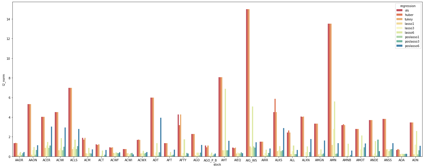
According to the grouped histogram above, in many cases positive Lasso with 1 or 3 non-zero betas are most robust amongst all regression types. More generally, we observe (in robustness) the following order

1. Positive Lasso with 1 or 3 non-zero betas
2. Regular Lasso with 1 or 3 non-zero betas
3. Regular Lasso with 6 non-zero betas
4. Positive Lasso with 6 non-zero betas
5. Tukey, Huber and OLS are giving visually same robustness

The last three regression come really similar which is out of our expectation. In contrast, the improvement of Lasso is significant, both without and with restriction of positive betas. We are seeing some improvement of over 90% decreases in L2 norm of beta differences from in-sample to out-of-sample regression, which directly describes the robustness of the underlying regression.

Box Plot

In addition to the histogram, we may also drop the individual stocks’ info and go one step further, by taking a look at the box plots.

1
2
3
4
5

fig = plt.figure()
ax = fig.add_subplot(111)
sns.boxplot(x='regression', y='l2_norm', ax=ax, data=temp, palette='Spectral')
plt.tight_layout()
plt.show()

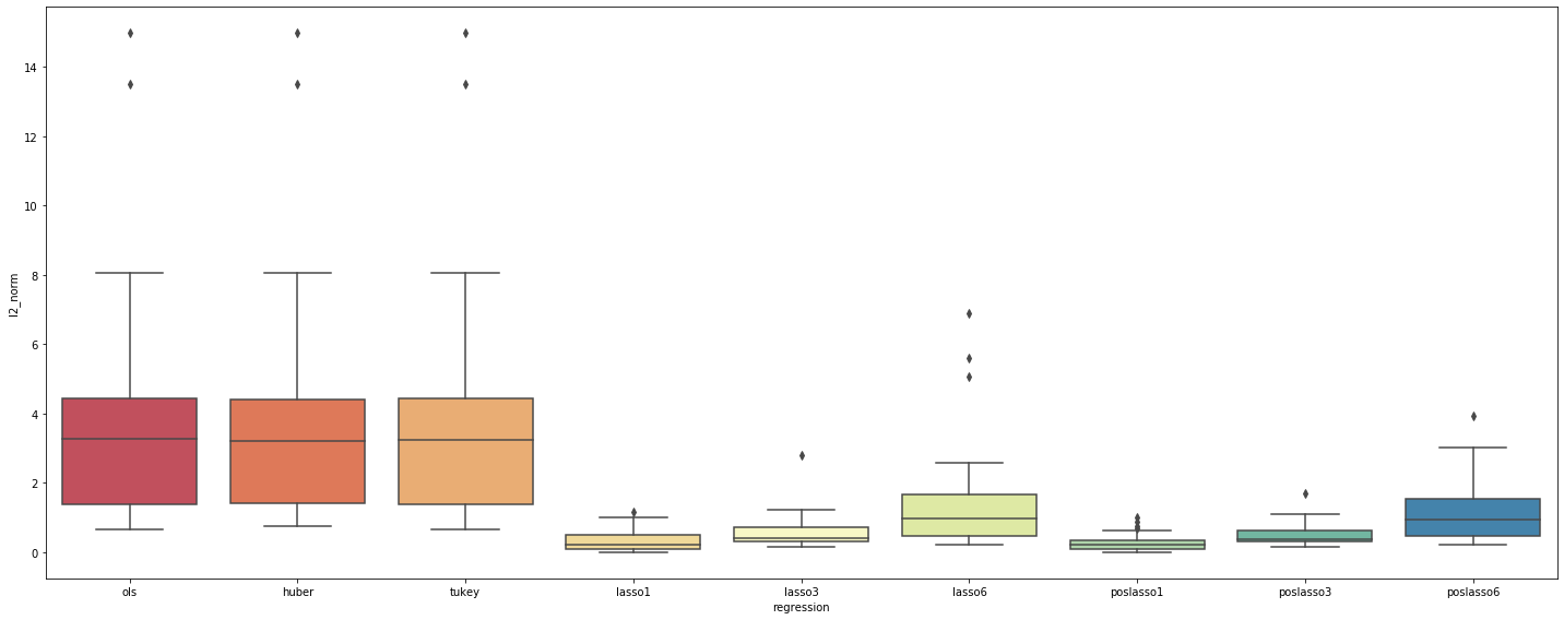
Box plot above gives a statistically speaking more summarized view on the overall robustness of the regressions. Now that we’ve excluded the idiosyncratic differences in this plot, the regressions robustness order becomes more clear:

1. Lasso (both with and without positive beta restriction) with 1 or 3 non-zero betas
2. Lasso (both with and without positive beta restriction) with 6 non-zero betas
3. OLS, Tukey and Huber

where the last three are the least robust, both from the dispersion of the L2 norm values and from the greater means (and outliers).

Talking about outliers, we do notice there’re some non-trivial advantage of having fewer non-zero betas: Lasso (both with and without positive beta restriction) with 1 non-zero beta is better than 3 and then 6 in that its outliers are visually smaller and closer to distribution means. While lasso6 and poslasso6 above are giving “extremer” extremes, the outliers given by lasso1 and poslasso1 are just trivial enough for us to make this conclusion.

Dist Plot

Another observation comes from the skewness of the above distributions. One may easily notice that all distributions are skewed toward the same direction: positive. We may get it verified by running skewness tests but rather let us just plot them here.

 1
 2
 3
 4
 5
 6
 7
 8
 9
10
11
12
13
14
15

g = sns.FacetGrid(temp, row='regression', hue='regression', aspect=15, height=1, palette='ocean')
g.map(sns.kdeplot, 'l2_norm', clip_on=False, shade=True, alpha=1, lw=1.5, bw=.2)
g.map(plt.axhline, y=0, lw=2, clip_on=False)

def label(x, color, label):
    ax = plt.gca()
    ax.text(0, .2, label, fontweight='normal', color=color, ha='left', va='center', transform=ax.transAxes)

g.map(label, 'l2_norm')
g.fig.subplots_adjust(hspace=-.25)
g.set_titles('')
g.set(yticks=[])
g.despine(bottom=True, left=True)
plt.tight_layout()
plt.show()

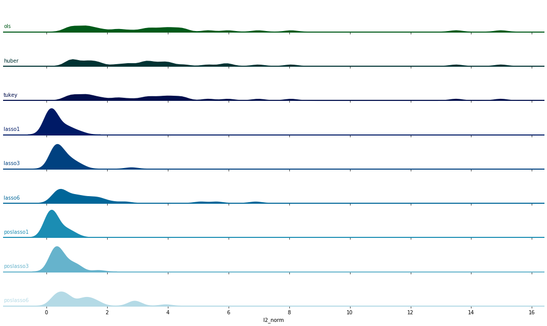
The dist plot above coincides with our observation: the right tail is much longer and fatter than left.