Comparison Between Exponential Weighted and Rolling Regression

This research discusses two normal prediction ways people are using: exponential weighted regression and rolling regression. By comparing the prediction errors of both ways, we generally get the idea of the difference between these two regressions.

1. Introduction

Comparison between two ways of regression

• Exponential Weighted Moving Regression: considering all the previous data to do the regression, however, following the intuition that the nearer data have more effects on the future data, the weight of data are different regarding time. Time decay applies here.
• Rolling Regression: for each date, we determine a moving boxcar window so that our prediction is based on a certain range of past data. The disadvantage of this method is that it could not smoothly decay old data and sometimes when an outlier is added or discarded, the prediction will change a lot.

Benchmark

We set the out-of-sample regression coefficient here as our benchmark to see which way of regression could give us a better prediction (lower prediction errors).

Another thing worth mentioning is that we’re using SPY(S&P 500 ETF Trust) to do the regression and prediction.

2. Data Preparation

Introduction of the packages in the research

We’re using several really important python pac

• Pandas: dataframe manipulation
• NumPy: support for mathematical functions and computation of arrays and matrics
• Quandl: source of our financial data
• Statsmodel: statistical analysis
• Matplotlib: plot tools
• tqdm: progress bar
• os: interact with the operating system
• PandasRollingOLS: package for computing rolling regression and obtain the coefficients

 1
 2
 3
 4
 5
 6
 7
 8
 9
10

import numpy as np
import pandas as pd
import quandl
import warnings
from tqdm.auto import tqdm
import matplotlib.pyplot as plt
import pickle
import os
from pyfinance.ols import PandasRollingOLS
import statsmodels.formula.api as smf

1
2
3

quandl.ApiConfig.api_key = 'yFs2mPKxvfCC26C4vG3K'
warnings.filterwarnings("ignore")
plt.rcParams['figure.figsize'] = (10, 5)

Obtaining data

Get the list of tickers that Quandl has and filter the tickers that could satisfy our conditions: tickers which have valid records from 2016-01-04 to 2019-12-31.

1
2
3
4

ticker = pd.read_csv('../HW5/ticker_list.csv')
ticker
ticker_list = ticker['Ticker']
ticker_list

0          A
1         AA
2       AAAU
3       AACG
4       AADR
        ... 
8627     ZUO
8628     ZVO
8629    ZYME
8630    ZYNE
8631    ZYXI
Name: Ticker, Length: 8632, dtype: object

For the tickers we selected, compute the daily return using daily Adjusted Closing Price.

 1
 2
 3
 4
 5
 6
 7
 8
 9
10
11
12
13
14
15
16
17

start_date = pd.to_datetime('2016-01-04')
end_date = pd.to_datetime('2019-12-31')

def get_eod(tic):
    adj_close = quandl.get(
        f'EOD/{tic}',
        start_date=start_date - pd.offsets.BDay(5),
        end_date=end_date + pd.offsets.BDay(5),
        column_index='11'
    ).Adj_Close
    assert adj_close.index[0] < start_date, f'start date too late: {adj_close.index[0]}'
    assert adj_close.index[-1] > end_date, f'end date too early: {adj_close.index[-1]}'
    daily_return = adj_close.pct_change().iloc[1:]
    daily_return.name = tic
    ret = daily_return[start_date:end_date]
    assert len(ret) == 1006  # length of SPY returns
    return ret

Also, add SPY into the EOD list.

 1
 2
 3
 4
 5
 6
 7
 8
 9
10
11
12
13
14
15
16
17
18
19
20
21

if os.path.isfile('EOD.pkl'):
    with open('EOD.pkl', 'rb') as f:
        EOD = pickle.load(f)
else:
    EOD = {}
    while len(EOD) <= 200:
        tic = np.random.choice(ticker_list, size=1)[0]
        if tic not in EOD.keys():
            try:
                EOD[tic] = get_eod(tic)
                msg = f'Current number of tickers: {len(EOD)}'
                print(f'{msg:<100}', end='\r')
            except Exception as e:
                msg = f'Skip {tic}: {e}'
                print(f'{msg:<100}', end='\r')
                continue
    
    with open('EOD.pkl', 'wb') as f:
        pickle.dump(EOD, f)

EOD['SPY'] = get_eod('SPY')

Current number of tickers: 201                                                                      

3. Computation of regressions

Exponential weighted regression

For the exponential weighted regression, we set $\frac{1}{\lambda}$ to be the characteristic time of our averaging, so $\alpha = 1 - e^{-\lambda \delta t}$ is the smoothing factor. Since our data is daily, $\delta t$ = 1.

By using the relationship between those variables, we set two functions in order to calculate our $\alpha$ and window given $\lambda$.

1
2
3
4
5

def lambda_to_alpha(lam):
    return 1 - np.exp(-lam)

def lambda_to_window(lam):
    return round(2 / lam)

Just for example, we choose $\lambda$ = 0.01.

1
2
3
4
5

lam = 0.01
alpha = lambda_to_alpha(lam)
window = lambda_to_window(lam)
assert window <= 300
lam, alpha, window

(0.01, 0.009950166250831893, 200)

Compute exponential-weighted coefficient.

1
2
3
4
5
6
7
8
9

EW_COEF = {}
SPY_VAR = EOD['SPY'].ewm(alpha=alpha, adjust=True).var()[1:]

for tic in tqdm(EOD):
    if tic != 'SPY':
        temp = pd.concat([EOD[tic], EOD['SPY']], axis=1)
        temp_cov = temp.ewm(alpha=alpha, adjust=True).cov()[tic].xs('SPY', level=1)[1:]
        temp_coef = temp_cov / SPY_VAR
        EW_COEF[tic] = temp_coef

In-Sample Rolling Regression

Given the lambda we have, window size = 200 here.

 1
 2
 3
 4
 5
 6
 7
 8
 9
10
11
12
13
14
15

time_list = ['2018-06-29', '2018-12-31', '2019-06-28', '2019-11-29']
time_list = [pd.to_datetime(t) for t in time_list]

ew_beta = {}
for tic in EW_COEF:
    temp = EW_COEF[tic].loc[time_list]
    ew_beta[tic] = temp

rolling_coef_b = {}
for tic in EOD:
    if tic != 'SPY':
        model = PandasRollingOLS(y=EOD[tic], x=EOD['SPY'], window=window)
        beta = model.beta.loc[time_list]['feature1']
        beta.name = tic
        rolling_coef_b[tic] = beta

Out-of-sample regression

1
2
3

# According to the time list, set the future 20-day time list 
time_list_2 = [t + pd.offsets.BDay(20) for t in time_list]
time_list_2

[Timestamp('2018-07-27 00:00:00'),
 Timestamp('2019-01-28 00:00:00'),
 Timestamp('2019-07-26 00:00:00'),
 Timestamp('2019-12-27 00:00:00')]

1
2
3
4
5
6
7
8

# Compute rolling regression for the future 20 days (which is our benchmark here)
rolling_coef_c = {}
for tic in EOD:
    if tic != 'SPY':
        model = PandasRollingOLS(y=EOD[tic], x=EOD['SPY'], window=20)
        beta = model.beta.loc[time_list]['feature1']
        beta.name = tic
        rolling_coef_c[tic] = beta

4. Statistical Comparison

To compare the performance of the above two regressions, I used several ways.

Comparison of MAE and MSE of the prediction

• MAE: MAE measures the average magnitude of the errors in a set of predictions
• MSE: MSE measures the average magnitude of the error

For both indexes, the smaller, the more accurate the prediction is.

1
2
3

y = np.array(list(map(list, rolling_coef_c.values())))
y_pred_ew = np.array(list(map(list, ew_beta.values())))
y_pred_wd = np.array(list(map(list, rolling_coef_b.values())))

1
2
3
4
5
6

mae_ew = abs(y - y_pred_ew).mean()
mae_wd = abs(y - y_pred_wd).mean()
mse_ew = ((y - y_pred_ew)**2).mean()
mse_wd = ((y - y_pred_wd)**2).mean()
print('For exponential-weighted regression, the prediction\'s MAE={:.4f}, MSE={:.4f};\n'
      'For rolling regression, the prediction\'s MAE={:.4f}, MSE={:.4f}'.format(mae_ew, mse_ew, mae_wd, mse_wd))

For exponential-weighted regression, the prediction's MAE=0.5353, MSE=1.1382;
For rolling regression, the prediction's MAE=0.5587, MSE=1.1956

From the result, we could see that the exponential-wegithed regression’s MAE and MSE are both smaller than that of rolling regression, which means the in this case, the exponential weighted regression is preferred.

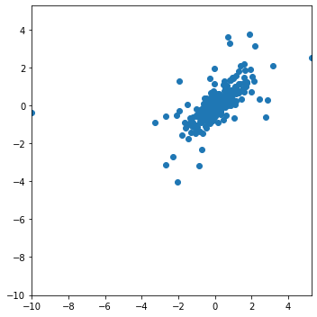
Relationship between beta(from exponential regression) and b(from rolling regression)

Drawing the scatter plot of the two regressions’ prediction erros of all the tickers by the two different regression, I tried to see if there’s any relationships between those two predictions’ errors.

1
2
3
4

df_coef = pd.DataFrame({'c': y.flatten(),
              'beta': y_pred_ew.flatten(),
              'b': y_pred_wd.flatten()})
df_coef

1
2
3
4
5
6
7
8

error = pd.DataFrame({
    'abs_err_beta': abs(df_coef['c'] - df_coef['beta']),
    'abs_err_b': abs(df_coef['c'] - df_coef['b']),
    'err_beta': df_coef['c'] - df_coef['beta'],
    'err_b': df_coef['c'] - df_coef['b']
})

error

1
2
3
4
5
6
7
8
9

error_min = min(error['err_b'].min(), error['err_beta'].min())
error_max = max(error['err_b'].max(), error['err_beta'].max())

fig = plt.figure(figsize=(5, 5))
plt.scatter(error['err_b'], error['err_beta'])
plt.xlim(error_min, error_max)
plt.ylim(error_min, error_max)
plt.tight_layout()
plt.show()

By checking the scatter plot, we could see that they’re forming a almost linear relationship. Because of this, we run a regression between those two coefficients’ prediction errors to see the coefficient of the regression.

1
2

regression_model = smf.ols('err_beta ~ err_b + 1', data=error).fit()
print(regression_model.summary())

                                 OLS Regression Results                                
=======================================================================================
Dep. Variable:               err_beta   R-squared (uncentered):                   0.994
Model:                            OLS   Adj. R-squared (uncentered):              0.994
Method:                 Least Squares   F-statistic:                          1.386e+05
Date:                Thu, 14 May 2020   Prob (F-statistic):                        0.00
Time:                        16:30:22   Log-Likelihood:                          880.22
No. Observations:                 804   AIC:                                     -1758.
Df Residuals:                     803   BIC:                                     -1754.
Df Model:                           1                                                  
Covariance Type:            nonrobust                                                  
==============================================================================
                 coef    std err          t      P>|t|      [0.025      0.975]
------------------------------------------------------------------------------
err_b          0.9729      0.003    372.315      0.000       0.968       0.978
==============================================================================
Omnibus:                       83.087   Durbin-Watson:                   2.752
Prob(Omnibus):                  0.000   Jarque-Bera (JB):              354.569
Skew:                           0.376   Prob(JB):                     1.01e-77
Kurtosis:                       6.165   Cond. No.                         1.00
==============================================================================

Warnings:
[1] Standard Errors assume that the covariance matrix of the errors is correctly specified.

From the result, we could see that the cofficient of the regression is almost 1, which means the prediction error of the two regressions are very close. However, since it’s still not 1, we could get the relationship that Error_exponential = 0.9729 * Error_rolling. So, the exponential regression is more accurate here.

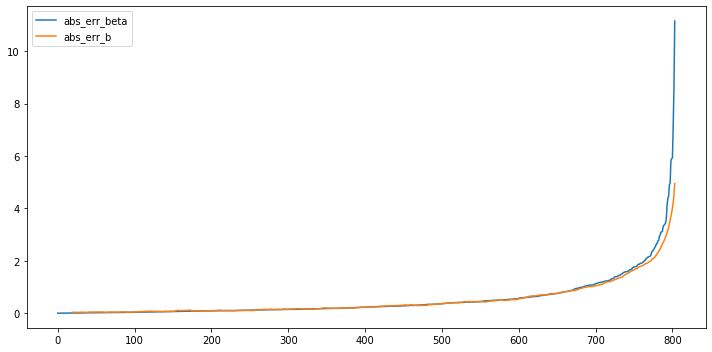
Plot of the absolute error of two regressions.

By sorting the absolute value of exponential regression model and then plot the prediction errors of those two regressions, we could tell that the result are pretty close. The only obvious difference is when absolute error of exponential weighted regression is extremely high, the absolute error of rolling regression is lower.

1
2
3
4
5

error = error.sort_values('abs_err_beta').reset_index(drop=True)
error['abs_err_b'] = error['abs_err_b'].rolling(20).mean()
error[['abs_err_beta', 'abs_err_b']].plot()
plt.tight_layout()
plt.show()

5. Play with more $\lambda s$

Using only one lambda is pretty limited here. So we dig into the exploration and try different lambda (different windows) here to see if there’re any patterns behind it.

Following, I chose $\lambda$ = 0.07, 0.05, 0.03 and 0.009. The corresponding window for the rolling regression here is: 29, 47, 60, 222.

In order to make the computation easier, I rewrote the above code and make it a function which takes $\lambda$ as input.

  1
  2
  3
  4
  5
  6
  7
  8
  9
 10
 11
 12
 13
 14
 15
 16
 17
 18
 19
 20
 21
 22
 23
 24
 25
 26
 27
 28
 29
 30
 31
 32
 33
 34
 35
 36
 37
 38
 39
 40
 41
 42
 43
 44
 45
 46
 47
 48
 49
 50
 51
 52
 53
 54
 55
 56
 57
 58
 59
 60
 61
 62
 63
 64
 65
 66
 67
 68
 69
 70
 71
 72
 73
 74
 75
 76
 77
 78
 79
 80
 81
 82
 83
 84
 85
 86
 87
 88
 89
 90
 91
 92
 93
 94
 95
 96
 97
 98
 99
100
101
102
103
104
105
106
107
108

def coef_comparison(lam):
    
    # Functions to obtain alpha and window regarding different lambdas
    def lambda_to_alpha(lam):
        return 1 - np.exp(-lam)
    
    def lambda_to_window(lam):
        return round(2 / lam)

    
    alpha = lambda_to_alpha(lam)
    window = lambda_to_window(lam)
    assert window <= 300
    
    
    # Compute exponential-weighted coefficient
    EW_COEF = {}
    SPY_VAR = EOD['SPY'].ewm(alpha=alpha, adjust=True).var()[1:]
    
    for tic in tqdm(EOD):
        if tic != 'SPY':
            temp = pd.concat([EOD[tic], EOD['SPY']], axis=1)
            temp_cov = temp.ewm(alpha=alpha, adjust=True).cov()[tic].xs('SPY', level=1)[1:]
            temp_coef = temp_cov / SPY_VAR
            EW_COEF[tic] = temp_coef
    
    
    # Build time-list of the four specific dates
    time_list = ['2018-06-29', '2018-12-31', '2019-06-28', '2019-11-29']
    time_list = [pd.to_datetime(t) for t in time_list]
    
    
    # Find the four specific dates' exponential-weighted beta
    ew_beta = {}
    for tic in EW_COEF:
        temp = EW_COEF[tic].loc[time_list]
        ew_beta[tic] = temp
        
    # Compute the rolling regression
    rolling_coef_b = {}
    for tic in EOD:
        if tic != 'SPY':
            model = PandasRollingOLS(y=EOD[tic], x=EOD['SPY'], window=window)
            beta = model.beta.loc[time_list]['feature1']
            beta.name = tic
            rolling_coef_b[tic] = beta
            
    # According to the time list, set the future 20-day time list 
    time_list_2 = [t + pd.offsets.BDay(20) for t in time_list]
    
    # Compute rolling regression for the future 20 days (which is our benchmark here)
    rolling_coef_c = {}
    for tic in EOD:
        if tic != 'SPY':
            model = PandasRollingOLS(y=EOD[tic], x=EOD['SPY'], window=20)
            beta = model.beta.loc[time_list]['feature1']
            beta.name = tic
            rolling_coef_c[tic] = beta
            
    # Convert the coefficients' values into seperate arrays           
    y = np.array(list(map(list, rolling_coef_c.values())))
    y_pred_ew = np.array(list(map(list, ew_beta.values())))
    y_pred_wd = np.array(list(map(list, rolling_coef_b.values())))
    
    # Calculate the MAE and MSE of the two predictions in order to compare them
    mae_ew = abs(y - y_pred_ew).mean()
    mae_wd = abs(y - y_pred_wd).mean()
    mse_ew = ((y - y_pred_ew)**2).mean()
    mse_wd = ((y - y_pred_wd)**2).mean()
    print('For exponential-weighted regression, the prediction\'s MAE={:.4f}, MSE={:.4f};\n'
          'For rolling regression, the prediction\'s MAE={:.4f}, MSE={:.4f}'.format(mae_ew, mse_ew, mae_wd, mse_wd))
    
    # Create a dataframe of the three different coefficients
    df_coef = pd.DataFrame({'c': y.flatten(),
                  'beta': y_pred_ew.flatten(),
                  'b': y_pred_wd.flatten()})

    # Create a dataframe of the prediction errors of the two predictions
    error = pd.DataFrame({
        'abs_err_beta': abs(df_coef['c'] - df_coef['beta']),
        'abs_err_b': abs(df_coef['c'] - df_coef['b']),
        'err_beta': df_coef['c'] - df_coef['beta'],
        'err_b': df_coef['c'] - df_coef['b']
    })
    
    # Scatter plot
    error_min = min(error['err_b'].min(), error['err_beta'].min())
    error_max = max(error['err_b'].max(), error['err_beta'].max())
    
    fig = plt.figure(figsize=(5, 5))
    plt.scatter(error['err_b'], error['err_beta'])
    plt.xlim(error_min, error_max)
    plt.ylim(error_min, error_max)
    plt.tight_layout()
    plt.show()
    
    # Regression between two errors
    regression_model = smf.ols('err_beta ~ err_b + 1', data=error).fit()
    print(regression_model.summary())
    
    # Plot the prediction erros
    error = error.sort_values('abs_err_beta').reset_index(drop=True)
    error['abs_err_b'] = error['abs_err_b'].rolling(20).mean()
    error[['abs_err_beta', 'abs_err_b']].plot()
    plt.title('Lambda={}, Window={}'.format(lam, window))
    plt.tight_layout()
    plt.show()
    

$\lambda$ = 0.07, window = 29

1

coef_comparison(0.07)

For exponential-weighted regression, the prediction's MAE=0.3028, MSE=0.3219;
For rolling regression, the prediction's MAE=0.3434, MSE=0.4840

                            OLS Regression Results                            
==============================================================================
Dep. Variable:               err_beta   R-squared:                       0.372
Model:                            OLS   Adj. R-squared:                  0.371
Method:                 Least Squares   F-statistic:                     475.0
Date:                Thu, 14 May 2020   Prob (F-statistic):           4.50e-83
Time:                        19:08:53   Log-Likelihood:                -498.01
No. Observations:                 804   AIC:                             1000.
Df Residuals:                     802   BIC:                             1009.
Df Model:                           1                                         
Covariance Type:            nonrobust                                         
==============================================================================
                 coef    std err          t      P>|t|      [0.025      0.975]
------------------------------------------------------------------------------
Intercept      0.0012      0.016      0.076      0.939      -0.030       0.032
err_b          0.4976      0.023     21.795      0.000       0.453       0.542
==============================================================================
Omnibus:                      484.829   Durbin-Watson:                   2.069
Prob(Omnibus):                  0.000   Jarque-Bera (JB):            25718.642
Skew:                           1.999   Prob(JB):                         0.00
Kurtosis:                      30.418   Cond. No.                         1.44
==============================================================================

Warnings:
[1] Standard Errors assume that the covariance matrix of the errors is correctly specified.

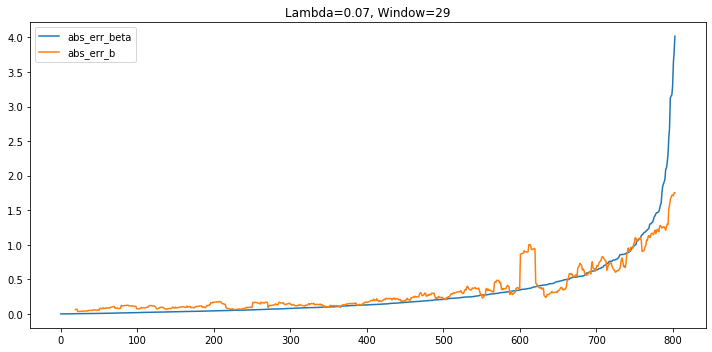
From the scatter plot and also the regression summary, we could see that the prediction errors of the two regressions are less linear correlated. After plotting the prediction errors, from the plot, we could see that for most of the time, the absolute error of rolling regression is higher and the exponential weighted regression’s prediction is more accurate (as the MAE and MSE shows).

$\lambda$ = 0.05, window = 40

1

coef_comparison(0.05)

For exponential-weighted regression, the prediction's MAE=0.3741, MSE=0.5525;
For rolling regression, the prediction's MAE=0.4540, MSE=0.7896

                            OLS Regression Results                            
==============================================================================
Dep. Variable:               err_beta   R-squared:                       0.878
Model:                            OLS   Adj. R-squared:                  0.878
Method:                 Least Squares   F-statistic:                     5796.
Date:                Thu, 14 May 2020   Prob (F-statistic):               0.00
Time:                        17:26:21   Log-Likelihood:                -54.356
No. Observations:                 804   AIC:                             112.7
Df Residuals:                     802   BIC:                             122.1
Df Model:                           1                                         
Covariance Type:            nonrobust                                         
==============================================================================
                 coef    std err          t      P>|t|      [0.025      0.975]
------------------------------------------------------------------------------
Intercept     -0.0062      0.009     -0.678      0.498      -0.024       0.012
err_b          0.7845      0.010     76.131      0.000       0.764       0.805
==============================================================================
Omnibus:                      828.136   Durbin-Watson:                   1.963
Prob(Omnibus):                  0.000   Jarque-Bera (JB):           245095.795
Skew:                           4.105   Prob(JB):                         0.00
Kurtosis:                      88.140   Cond. No.                         1.14
==============================================================================

Warnings:
[1] Standard Errors assume that the covariance matrix of the errors is correctly specified.

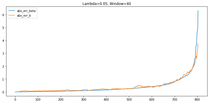
Things are very similar with the previous one. Here, for most of the time, the prediction error of rolling regression is higher than that of exponential regression. However, the difference between the two mothods are shrinking.

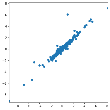
$\lambda$ = 0.03, window = 67

1

coef_comparison(0.03)

For exponential-weighted regression, the prediction's MAE=0.4600, MSE=0.8762;
For rolling regression, the prediction's MAE=0.5081, MSE=0.9748

                            OLS Regression Results                            
==============================================================================
Dep. Variable:               err_beta   R-squared:                       0.925
Model:                            OLS   Adj. R-squared:                  0.925
Method:                 Least Squares   F-statistic:                     9962.
Date:                Thu, 14 May 2020   Prob (F-statistic):               0.00
Time:                        17:27:46   Log-Likelihood:                -42.657
No. Observations:                 804   AIC:                             89.31
Df Residuals:                     802   BIC:                             98.69
Df Model:                           1                                         
Covariance Type:            nonrobust                                         
==============================================================================
                 coef    std err          t      P>|t|      [0.025      0.975]
------------------------------------------------------------------------------
Intercept      0.0124      0.009      1.372      0.171      -0.005       0.030
err_b          0.9116      0.009     99.809      0.000       0.894       0.930
==============================================================================
Omnibus:                     1403.599   Durbin-Watson:                   2.011
Prob(Omnibus):                  0.000   Jarque-Bera (JB):          1510276.440
Skew:                          11.096   Prob(JB):                         0.00
Kurtosis:                     214.164   Cond. No.                         1.04
==============================================================================

Warnings:
[1] Standard Errors assume that the covariance matrix of the errors is correctly specified.

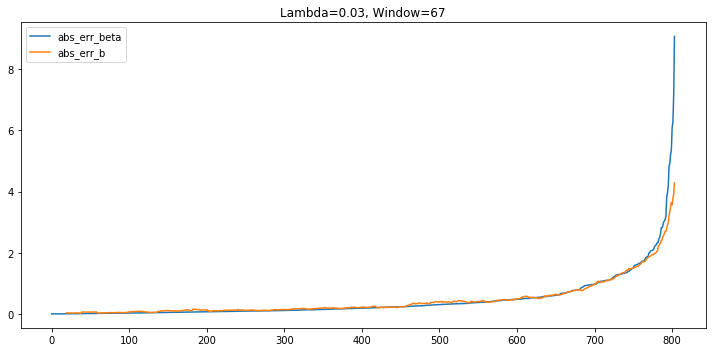
As the window is widening, rolling regression is improving. However, exponential weighted regression is still preferred here.

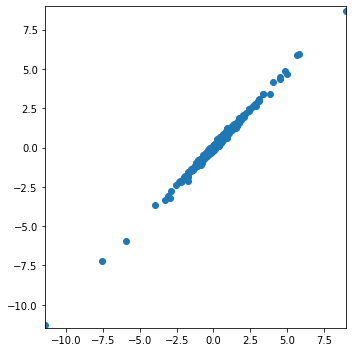
$\lambda$ = 0.009, window = 222

1

coef_comparison(0.009)

For exponential-weighted regression, the prediction's MAE=0.5388, MSE=1.1476;
For rolling regression, the prediction's MAE=0.5571, MSE=1.1940

                            OLS Regression Results                            
==============================================================================
Dep. Variable:               err_beta   R-squared:                       0.995
Model:                            OLS   Adj. R-squared:                  0.995
Method:                 Least Squares   F-statistic:                 1.503e+05
Date:                Thu, 14 May 2020   Prob (F-statistic):               0.00
Time:                        17:25:35   Log-Likelihood:                 910.91
No. Observations:                 804   AIC:                            -1818.
Df Residuals:                     802   BIC:                            -1808.
Df Model:                           1                                         
Covariance Type:            nonrobust                                         
==============================================================================
                 coef    std err          t      P>|t|      [0.025      0.975]
------------------------------------------------------------------------------
Intercept      0.0007      0.003      0.241      0.810      -0.005       0.006
err_b          0.9777      0.003    387.675      0.000       0.973       0.983
==============================================================================
Omnibus:                       85.769   Durbin-Watson:                   2.566
Prob(Omnibus):                  0.000   Jarque-Bera (JB):              580.498
Skew:                          -0.152   Prob(JB):                    8.84e-127
Kurtosis:                       7.152   Cond. No.                         1.11
==============================================================================

Warnings:
[1] Standard Errors assume that the covariance matrix of the errors is correctly specified.

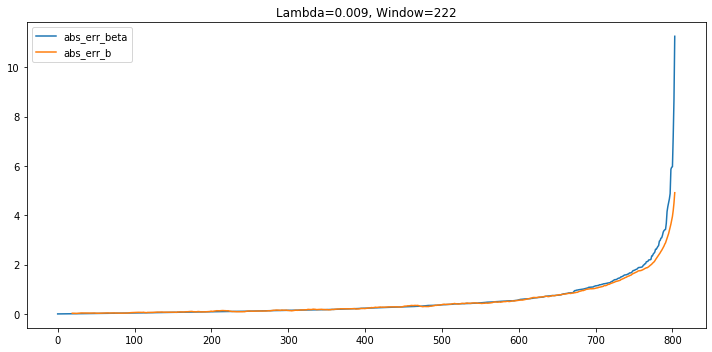
Most of the time, the performance of the two regressions are very close. Except for the extreme case when the error of exponential weighted regression is high, then the rolling regression is more preferred.

6. Conclusion

From the performances we get above, we could conclude that overall, the performance of exponential weighted regression is better and the prediction is more accurate. The limitation of the rolling regression is that comparing with exponential weighted regression, the information it gets is not enough. So, as the $\lambda$ gets smaller, which implies the window of the rolling regression is larger, the performance is better and closer to exponential weighted regression, which suggests us that in order to improve the rolling regression, we should widen the window.

However, we could not just widen our window unlimitedly. The edge of rolling regression is that its more reactive and responsive to the real-time market change. When something huge happens, it will immediately reflect on the regression and the prediction. When the window of rolling regression is larger, the effect of real-time information will be smaller, which is not good for activities such as high-frequency trading.