This is a strategy which we trade different securities by ranking their performance and using their quantile as signals.
1. Data preparation
Introduction of the packages we used
We’re using several really important python packages in this strategy:
- Pandas: dataframe manipulation
- NumPy: support for mathematical functions and computation of arrays and matrics
- Quandl: source of our future data
- Statsmodel: statistical analysis
- Matplotlib: plot tools
- Seaborn: statistical data visualization
- Glob: retrieve files matching a specified pattern
- os: interact with the operating system
- tqdm: progress bar
 1
 2
 3
 4
 5
 6
 7
 8
 9
10
11
12
13
14
|
import os
import numpy as np
import pandas as pd
import pickle
import quandl
import warnings
from functools import reduce
from tqdm.auto import tqdm
import matplotlib.pyplot as plt
import statsmodels.formula.api as smf

pd.set_option('display.max_rows', 20)
warnings.filterwarnings("ignore")
plt.rcParams['figure.figsize'] = (10, 5)
|
Data Cleaning
We load our ZFB and EOD datasets from Quandl in this part, including a strict filteration process that only keeps:
- EOD adjusted closing prices are available
- Maximum of debt/market cap ratio is greater3 than 0.1
- Not in automotive, financial or insurance sector
- No more than one year old as determined by filing dates
We set the constant funding rate as 0 in our strategy.
Import ZFB
 1
 2
 3
 4
 5
 6
 7
 8
 9
10
11
12
13
14
15
16
17
18
19
20
21
22
23
24
25
26
27
28
29
30
31
32
33
34
35
36
37
38
39
40
41
|
keys = ['ticker', 'per_end_date']
z1 = pd.read_csv('ZACKS_1.csv', usecols=keys + ['mkt_val'])
cols = ['nbr_shares_out', 'filing_date', 'net_lterm_debt', 'tot_lterm_debt', 'per_type',
        'eps_diluted_net', 'basic_net_eps', 'zacks_sector_code', 'zacks_x_ind_code']
z2 = pd.read_csv('ZACKS_5.csv', usecols=keys + cols)
z3 = pd.read_csv('ZACKS_3.csv', usecols=keys + ['tot_debt_tot_equity', 'per_type', 'ret_invst'])

def f(x):
    assert len(x) <= 2
    if len(x) == 2:
        x = x[x.per_type=='Q'].fillna(x[x.per_type=='A'])
    return x.reset_index().drop(['index', 'ticker', 'per_type', 'per_end_date'], axis=1)

zacks = {}

for tic in tqdm(set(z1['ticker'])):
    temp1 = z1[z1.ticker==tic].drop('ticker', axis=1).set_index('per_end_date')

    temp2 = z2[z2.ticker==tic].groupby('per_end_date').apply(f)
    if len(temp2) == 0:
        continue
    temp2 = temp2.droplevel(1)

    temp3 = z3[z3.ticker==tic].groupby('per_end_date').apply(f)
    if len(temp3) == 0:
        continue
    temp3 = temp3.droplevel(1)

    temp = pd.concat([temp1, temp2, temp3], axis=1).sort_index()
    temp = temp['2012-01':'2020-01']
    temp['Debt_To_Mkt_Cap'] = temp['tot_debt_tot_equity'] / temp['mkt_val']
    temp['Debt_To_Mkt_Cap']['2012-09-30':'2012-09-30']
    zacks[tic] = temp

temp = pd.concat(zacks, keys=zacks).reset_index()
temp.drop([c for c in temp.columns if ':' in c], axis=1, inplace=True)
temp.columns = ['ticker'] + list(temp.columns[1:])
temp.to_csv('../HW4/zacks.csv')

ZFB = pd.read_csv('../HW4/zacks.csv', index_col=0)
ZFB
|
| id |
ticker |
per_end_date |
mkt_val |
zacks_sector_code |
zacks_x_ind_code |
filing_date |
nbr_shares_out |
basic_net_eps |
tot_lterm_debt |
net_lterm_debt |
eps_diluted_net |
tot_debt_tot_equity |
ret_invst |
Debt_To_Mkt_Cap |
| 0 |
DOOO |
2017-01-31 |
NaN |
5.0 |
10.0 |
NaN |
NaN |
0.91 |
NaN |
NaN |
0.91 |
NaN |
NaN |
NaN |
| 1 |
DOOO |
2017-04-30 |
NaN |
5.0 |
10.0 |
NaN |
NaN |
-0.13 |
NaN |
NaN |
-0.13 |
NaN |
NaN |
NaN |
| 2 |
DOOO |
2017-07-31 |
NaN |
5.0 |
10.0 |
NaN |
NaN |
0.68 |
NaN |
NaN |
0.67 |
NaN |
NaN |
NaN |
| 3 |
DOOO |
2017-10-31 |
NaN |
5.0 |
10.0 |
NaN |
NaN |
0.60 |
NaN |
NaN |
0.60 |
NaN |
NaN |
NaN |
| 4 |
DOOO |
2018-01-31 |
NaN |
5.0 |
10.0 |
NaN |
NaN |
0.89 |
752.750 |
NaN |
0.89 |
-17.2607 |
12.8604 |
NaN |
| … |
… |
… |
… |
… |
… |
… |
… |
… |
… |
… |
… |
… |
… |
… |
| 219351 |
NEFF |
2016-09-30 |
226.69 |
7.0 |
286.0 |
2016-10-26 |
23863590.0 |
NaN |
733.843 |
3.051 |
0.31 |
-4.8868 |
2.2996 |
-0.021557 |
| 219352 |
NEFF |
2016-12-31 |
335.72 |
7.0 |
286.0 |
2017-03-06 |
17885380.0 |
NaN |
691.391 |
-30.549 |
0.53 |
-5.2487 |
2.9126 |
-0.015634 |
| 219353 |
NEFF |
2017-03-31 |
463.20 |
7.0 |
286.0 |
2017-04-26 |
23814710.0 |
NaN |
677.773 |
-14.230 |
0.18 |
-5.4337 |
1.1278 |
-0.011731 |
| 219354 |
NEFF |
2017-06-30 |
453.04 |
7.0 |
286.0 |
2017-08-03 |
23844420.0 |
NaN |
680.271 |
-12.130 |
0.34 |
-6.0733 |
2.1708 |
-0.013406 |
| 219355 |
NEFF |
2017-09-30 |
596.11 |
NaN |
NaN |
NaN |
NaN |
NaN |
NaN |
NaN |
NaN |
NaN |
NaN |
NaN |
 1
 2
 3
 4
 5
 6
 7
 8
 9
10
11
|
ZFB['eps_diluted_net'].fillna(ZFB['basic_net_eps'], inplace=True)

con1 = ZFB[(ZFB['zacks_sector_code'] == 5)]
con2 = ZFB[(ZFB['zacks_sector_code'] == 13)]
con3 = ZFB[(ZFB['zacks_x_ind_code'].isin([85, 86, 87, 88, 89, 61, 62, 63, 64, 65, 66, 67 ,68 ,69, 282, 7, 8, 9, 10, 11, 82, 124, 210]))]  # filter industry
con4 = ZFB[((ZFB['basic_net_eps'].isna()) & (ZFB['eps_diluted_net'].isna()))]

ticker_out = set(pd.concat([con1, con2, con3, con4]).set_index('ticker').index)
ZFB_update = ZFB[~(ZFB['ticker'].isin(ticker_out))].set_index('ticker')

ticker_update = set(ZFB_update.index)
|
Import EOD from Quandl
 1
 2
 3
 4
 5
 6
 7
 8
 9
10
11
12
13
14
15
16
17
18
19
20
|
start_date = '2012-01-01'
end_date = '2019-01-31'
n = len(ticker_update)

def get_eod(tic):
    return quandl.get(f'EOD/{tic}', start_date=start_date, end_date=end_date)


if os.path.isfile('EOD.pkl'):
    with open('EOD.pkl', 'rb') as f:
        EOD = pickle.load(f)
else:
    EOD = {}
    for tic in tqdm(ticker_update):
        try:
            EOD[tic] = get_eod(tic)
        except Exception:
            print(f'skip {tic} as it\'s missing in EOD dataset')
    with open('EOD.pkl', 'wb') as f:
        pickle.dump(EOD, f)
|
Keep organizing data in order to make the merge of ZFB and EOD easier.
1
2
3
4
5
6
7
|
ticker_update2 = set(EOD) & ticker_update
ZFB_update2 = ZFB[(ZFB['ticker'].isin(ticker_update2))]
ZFB_update3 = ZFB_update2[ZFB_update2['tot_debt_tot_equity'] > 0.1]
ZFB_update3['final_debt'] = ZFB_update3['net_lterm_debt'].fillna(ZFB_update3['tot_lterm_debt'])
ZFB_update3['final_debt'] = ZFB_update3['final_debt'].fillna(0)
ZFB_update3['per_end_date'] = pd.to_datetime(ZFB_update3['per_end_date'])
ZFB_update3['filing_date'] = pd.to_datetime(ZFB_update3['filing_date'])
|
Calculate Financial Ratios
We’re going to use three different daily financial ratios to help us selcet tickers we’re gonna use in our strategy. The three ratios are:
- Debt to Market Cap: tot_debt_tot_equity * per_end_date_price / daily adjusted closing price
- Return on Investment: return_on_investment * (longterm_debt + market_value) / (longterm_debt + market_val * daily_adjusted_closing_price / per_end_date_price)
- Price to Earnings: daily_adjusted_closing_price / earnings_per_share
We calcuate the three daily ratios based on their filing date and also the period end date for each company. Also, to prepare for the backtest, here we put the three ratios and also the daily return in the same dataframe.
 1
 2
 3
 4
 5
 6
 7
 8
 9
10
11
12
13
14
15
16
17
18
19
20
21
22
23
24
25
26
27
28
29
30
31
32
33
34
35
36
37
38
39
40
41
42
43
44
45
46
47
48
49
50
51
52
53
54
55
|
cols = ['ticker', 'per_end_date', 'mkt_val', 'filing_date', 'eps_diluted_net',
        'tot_debt_tot_equity', 'ret_invst', 'final_debt']
ZFB_update4 = ZFB_update3[cols].set_index('ticker')

available_tickers = set()
for ticker in set(ZFB_update4.index):
    if 'Adj_Close' in EOD[ticker]:
        available_tickers.add(ticker)

from functools import lru_cache


@lru_cache(maxsize=None)
def prepare_data(ticker):
    ret = ZFB_update4.loc[ticker]
    if isinstance(ret, pd.Series): return
    ret = ret.set_index('per_end_date').join(EOD[ticker]['Adj_Close'], how='outer')
    ret['Adj_Close'] = ret['Adj_Close'].ffill()
    ret = ret.dropna(subset=['filing_date'], axis=0)
    ret.columns = list(ret.columns[:-1]) + ['Adj_Close_bench']
    ret = ret.reset_index(drop=True)
    ret = ret.set_index('filing_date')
    ret = EOD[ticker][['Adj_Close']].join(ret.shift(), how='left').ffill().dropna()
    return ret


def calculate_ratios(ticker):
    data = prepare_data(ticker)
    if data is None: return
    if not len(data): return
    d2m = data.eval('tot_debt_tot_equity * Adj_Close_bench / Adj_Close')
    roi = data.eval('ret_invst * (final_debt + mkt_val) / (final_debt + mkt_val * Adj_Close / Adj_Close_bench)')
    pe = data.eval('Adj_Close / eps_diluted_net')
    px = data['Adj_Close']
    res = pd.concat([d2m, roi, pe, px], axis=1)
    res.columns = ['d2m', 'roi', 'pe', 'px']
    return res

# calculate_ratios('LLY').loc['2017-10-27']

if os.path.isfile('RATIOS.pkl'):
    with open('RATIOS.pkl', 'rb') as f:
        RATIOS = pickle.load(f)
else:
    RATIOS = {}
    for ticker in tqdm(available_tickers):
        ratios = calculate_ratios(ticker)
        if ratios is None:
            continue
        else:
            RATIOS[ticker] = ratios
    with open('RATIOS.pkl', 'wb') as f:
        pickle.dump(RATIOS, f)

print(f'{len(RATIOS)} tickers in total')
|
1723 tickers in total
1
|
STRATEGY_DATA = {k: v.resample('M').last().pct_change() for k, v in RATIOS.items()}
|
2. Backtest
In this section, we perform the backtest for this strategy. We seperately consider each of the financial ratios we calculated earlier as the index in order to rank the performance of the companies in our portfolio. By using the rop-and-bottom strategy , we dynamically take a long position in the top 10 percentile of all companies’ stocks and a short position in the bottom 10 percentile.
Although we’re assuming that there’s no trading costs here and all securities are easy to borrow, since in the real world these fees are all gonna be the costs of our strategy, I decide to change my position every month in order to simulate the real world as close as possible.
Also, we introduce three indexes to help us find if the strategy is good, they’re:
- Sharpe Ratio: return of an investment compared to its risk
- Maximnm Drawdown: maximum observed loss from a peak to a trough
- Winning Rate: the percentage of winning
1
2
3
4
5
6
7
8
|
def sharpe(x):
    return x.mean() / (x.std() * 12**0.5 if x.std() else np.nan)

def win_rate(x):
    return sum(x > 0) / (sum(x != 0) if any(x != 0) else np.nan)

def maximum_drawdown(x):  # use absolute drawdown instead of percentage here -> cum pnl could be negative
    return (x.cummax() - x).max()
|
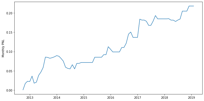
Following are the three seperate backtests for each of the financial ratio.
Debt_to_market_ratio
 1
 2
 3
 4
 5
 6
 7
 8
 9
10
11
12
13
14
15
16
17
18
19
20
21
22
23
24
25
|
debt_to_market_table = pd.concat([STRATEGY_DATA[tic]['d2m'] for tic in STRATEGY_DATA], axis=1)
debt_to_market_table.columns = STRATEGY_DATA.keys()
debt_to_market_table_temp = debt_to_market_table.T

n = round(1723 * 0.1)  # number of tickers we're gonna use in the strategy

returns_table = pd.concat([STRATEGY_DATA[tic]['px'] for tic in STRATEGY_DATA], axis=1)
returns_table.columns = STRATEGY_DATA.keys()

debt_to_market_strategy = pd.DataFrame(
    [debt_to_market_table_temp.nlargest(n, t).index.tolist() +
     debt_to_market_table_temp.nsmallest(n, t).index.tolist() for t in debt_to_market_table.index],
    index=debt_to_market_table.index).shift().dropna()

coef = np.array([1] * n + [-1] * n) / (2 * n)

debt_to_market_return = pd.Series([
    returns_table.loc[t, debt_to_market_strategy.loc[t].values] @ coef
    for t in debt_to_market_strategy.index
], index=debt_to_market_strategy.index)

plt.figure()
plt.plot(debt_to_market_return.fillna(0).cumsum())
plt.ylabel('Monthly PNL')
plt.tight_layout()
|

1
|
print(f'sharpe={sharpe(debt_to_market_return):.2f}, win%={win_rate(debt_to_market_return):.2%}, mdd={maximum_drawdown(debt_to_market_return):.2%}')
|
sharpe=0.03, win%=33.77%, mdd=7.43%
Return on Investment
 1
 2
 3
 4
 5
 6
 7
 8
 9
10
11
12
13
14
15
16
17
18
19
20
21
22
23
24
25
|
return_on_investment_table = pd.concat([STRATEGY_DATA[tic]['roi'] for tic in STRATEGY_DATA], axis=1)
return_on_investment_table.columns = STRATEGY_DATA.keys()
return_on_investment_table_temp = return_on_investment_table.T

n = round(1723 * 0.1)  # number of tickers we're gonna use in the strategy

returns_table = pd.concat([STRATEGY_DATA[tic]['px'] for tic in STRATEGY_DATA], axis=1)
returns_table.columns = STRATEGY_DATA.keys()

return_on_investment_strategy = pd.DataFrame(
    [return_on_investment_table_temp.nlargest(n, t).index.tolist() +
     return_on_investment_table_temp.nsmallest(n, t).index.tolist() for t in return_on_investment_table.index],
    index=return_on_investment_table.index).shift().dropna()

coef = np.array([1] * n + [-1] * n) / (2 * n)

return_on_investment_return = pd.Series([
    returns_table.loc[t, return_on_investment_strategy.loc[t].values] @ coef
    for t in return_on_investment_strategy.index
], index=return_on_investment_strategy.index)

plt.figure()
plt.plot(return_on_investment_return.fillna(0).cumsum())
plt.ylabel('Monthly PNL')
plt.tight_layout()
|
1
|
print(f'sharpe={sharpe(return_on_investment_return):.2f}, win%={win_rate(return_on_investment_return):.2%}, mdd={maximum_drawdown(return_on_investment_return):.2%}')
|
sharpe=0.10, win%=40.26%, mdd=5.80%
Price to Earnings
 1
 2
 3
 4
 5
 6
 7
 8
 9
10
11
12
13
14
15
16
17
18
19
20
21
22
23
24
25
|
price_to_earnings_table = pd.concat([STRATEGY_DATA[tic]['pe'] for tic in STRATEGY_DATA], axis=1)
price_to_earnings_table.columns = STRATEGY_DATA.keys()
price_to_earnings_table_temp = price_to_earnings_table.T

n = round(1723 * 0.1)  # number of tickers we're gonna use in the strategy

returns_table = pd.concat([STRATEGY_DATA[tic]['px'] for tic in STRATEGY_DATA], axis=1)
returns_table.columns = STRATEGY_DATA.keys()

price_to_earnings_strategy = pd.DataFrame(
    [price_to_earnings_table_temp.nlargest(n, t).index.tolist() +
     price_to_earnings_table_temp.nsmallest(n, t).index.tolist() for t in price_to_earnings_table.index],
    index=price_to_earnings_table.index).shift().dropna()

coef = np.array([1] * n + [-1] * n) / (2 * n)

price_to_earnings_return = pd.Series([
    returns_table.loc[t, price_to_earnings_strategy.loc[t].values] @ coef
    for t in price_to_earnings_strategy.index
], index=price_to_earnings_strategy.index)

plt.figure()
plt.plot(price_to_earnings_return.fillna(0).cumsum())
plt.ylabel('Monthly PNL')
plt.tight_layout()
|
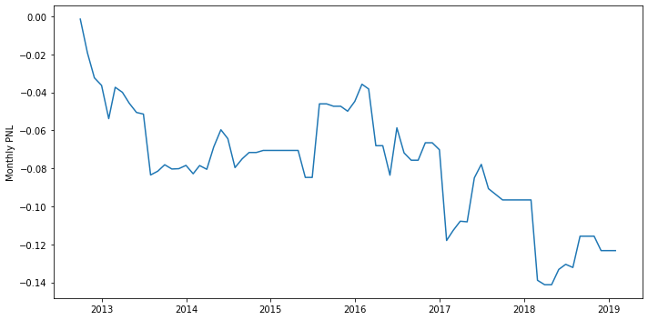
Here, from the plot of cumulative return of the strategy, we could find that the return is negative all the time. Reasonably, we could guess that maybe the correlation between the PE ratio and our monthly returns are negative so that our position here is wrong.
So, we could use a regression to analyze this special case here.\
First, we organize the three ratios and also the returns in one dataframe for the convenience of the regression
 1
 2
 3
 4
 5
 6
 7
 8
 9
10
|
def add_return(x):
    x['return'] = x['px'].shift()
    return x

STRATEGY_DATA_update = {k: add_return(v) for k, v in STRATEGY_DATA.items()}

regression_table = pd.concat([df[['return', 'd2m', 'roi', 'pe']].dropna() for df in STRATEGY_DATA_update.values()])
regression_table = regression_table[(abs(regression_table) <= 1e6).all(axis=1)]
regression_table.columns = ['ret', 'd2m', 'roi', 'pe']
regression_table
|
| time |
ret |
d2m |
roi |
pe |
| 2015-10-31 |
-0.208361 |
-0.190541 |
-0.173861 |
0.235393 |
| 2015-11-30 |
0.235393 |
-0.129454 |
-0.119475 |
0.148704 |
| 2015-12-31 |
0.148704 |
0.032284 |
0.029722 |
-0.031275 |
| 2016-01-31 |
-0.031275 |
0.184988 |
0.167840 |
-0.156110 |
| 2016-02-29 |
-0.156110 |
-0.173669 |
-0.160149 |
0.210169 |
| … |
… |
… |
… |
… |
| 2017-05-31 |
0.028055 |
0.060240 |
1.312317 |
-0.527728 |
| 2017-06-30 |
-0.032418 |
-0.110905 |
-0.114231 |
0.124740 |
| 2017-07-31 |
0.124740 |
0.042822 |
0.044163 |
-0.041064 |
| 2017-08-31 |
-0.041064 |
-0.125853 |
-0.686000 |
1.827308 |
| 2017-09-30 |
-0.057564 |
-0.126829 |
-0.139936 |
0.145251 |
1
2
|
result_regression = smf.ols('ret ~ pe + 0', data=regression_table).fit()
print(result_regression.summary())
|
                                 OLS Regression Results
=======================================================================================
Dep. Variable:                    ret   R-squared (uncentered):                   0.000
Model:                            OLS   Adj. R-squared (uncentered):              0.000
Method:                 Least Squares   F-statistic:                              5.982
Date:                Sat, 09 May 2020   Prob (F-statistic):                      0.0145
Time:                        10:04:11   Log-Likelihood:                          18935.
No. Observations:              106213   AIC:                                 -3.787e+04
Df Residuals:                  106212   BIC:                                 -3.786e+04
Df Model:                           1
Covariance Type:            nonrobust
==============================================================================
                 coef    std err          t      P>|t|      [0.025      0.975]
------------------------------------------------------------------------------
pe             0.0001    4.6e-05      2.446      0.014    2.23e-05       0.000
==============================================================================
Omnibus:                   394481.026   Durbin-Watson:                   2.025
Prob(Omnibus):                  0.000   Jarque-Bera (JB):     683351033378.908
Skew:                          80.866   Prob(JB):                         0.00
Kurtosis:                   12428.158   Cond. No.                         1.00
==============================================================================

Warnings:
[1] Standard Errors assume that the covariance matrix of the errors is correctly specified.
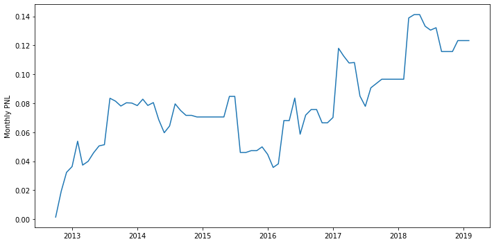
From the regression result, we could see that their correlation is nearly 0. So we try to change the original position of the strategy to opposite, which is to long the bottom stock and short the top stock.
 1
 2
 3
 4
 5
 6
 7
 8
 9
10
11
12
13
14
15
16
17
18
19
20
21
22
23
24
25
|
price_to_earnings_table = pd.concat([STRATEGY_DATA[tic]['pe'] for tic in STRATEGY_DATA], axis=1)
price_to_earnings_table.columns = STRATEGY_DATA.keys()
price_to_earnings_table_temp = price_to_earnings_table.T

n = round(1723 * 0.1)  # number of tickers we're gonna use in the strategy

returns_table = pd.concat([STRATEGY_DATA[tic]['px'] for tic in STRATEGY_DATA], axis=1)
returns_table.columns = STRATEGY_DATA.keys()

price_to_earnings_strategy = pd.DataFrame(
    [price_to_earnings_table_temp.nlargest(n, t).index.tolist() +
     price_to_earnings_table_temp.nsmallest(n, t).index.tolist() for t in price_to_earnings_table.index],
    index=price_to_earnings_table.index).shift().dropna()

coef = np.array([-1] * n + [1] * n) / (2 * n)

price_to_earnings_return = pd.Series([
    returns_table.loc[t, price_to_earnings_strategy.loc[t].values] @ coef
    for t in price_to_earnings_strategy.index
], index=price_to_earnings_strategy.index)

plt.figure()
plt.plot(price_to_earnings_return.fillna(0).cumsum())
plt.ylabel('Monthly PNL')
plt.tight_layout()
|
1
|
print(f'sharpe={sharpe(price_to_earnings_return):.2f}, win%={win_rate(price_to_earnings_return):.2%}, mdd={maximum_drawdown(price_to_earnings_return):.2%}')
|
sharpe=0.04, win%=42.86%, mdd=7.09%
It seems like the fix way of changing position works here.
If we use two indexes such as debt_to_market ratio and return on investment, the strategy is different from above. We should firstly take the regression of monthly returns and the combination of the two indexes in order to analyze the relationship between them. Once the correlation is fixed, we could use the regression to predict the return and then use the predicted return as our new index to rank the companies. Once the ranking is set, we could then use the signal to compute our top-and-bottom strategy.
Multiple indexes
1
2
3
|
debt_to_mkt_roi_table = pd.concat([df[['return', 'd2m', 'roi']].dropna() for df in STRATEGY_DATA_update.values()])
debt_to_mkt_roi_table = debt_to_mkt_roi_table[(abs(debt_to_mkt_roi_table) <= 1e6).all(axis=1)]
debt_to_mkt_roi_table
|
| time |
return |
d2m |
roi |
| 2015-10-31 |
-0.208361 |
-0.190541 |
-0.173861 |
| 2015-11-30 |
0.235393 |
-0.129454 |
-0.119475 |
| 2015-12-31 |
0.148704 |
0.032284 |
0.029722 |
| 2016-01-31 |
-0.031275 |
0.184988 |
0.167840 |
| 2016-02-29 |
-0.156110 |
-0.173669 |
-0.160149 |
| … |
… |
… |
… |
| 2017-05-31 |
0.028055 |
0.060240 |
1.312317 |
| 2017-06-30 |
-0.032418 |
-0.110905 |
-0.114231 |
| 2017-07-31 |
0.124740 |
0.042822 |
0.044163 |
| 2017-08-31 |
-0.041064 |
-0.125853 |
-0.686000 |
| 2017-09-30 |
-0.057564 |
-0.126829 |
-0.139936 |
1
2
|
result = smf.ols('ret ~ d2m + roi + 0', data=debt_to_mkt_roi_table).fit()
print(result.summary())
|
                                 OLS Regression Results
=======================================================================================
Dep. Variable:                    ret   R-squared (uncentered):                   0.000
Model:                            OLS   Adj. R-squared (uncentered):             -0.000
Method:                 Least Squares   F-statistic:                             0.2486
Date:                Sat, 09 May 2020   Prob (F-statistic):                       0.780
Time:                        03:57:33   Log-Likelihood:                          18932.
No. Observations:              106213   AIC:                                 -3.786e+04
Df Residuals:                  106211   BIC:                                 -3.784e+04
Df Model:                           2
Covariance Type:            nonrobust
==============================================================================
                 coef    std err          t      P>|t|      [0.025      0.975]
------------------------------------------------------------------------------
d2m         6.845e-08   1.99e-05      0.003      0.997   -3.89e-05     3.9e-05
roi         1.401e-05   1.99e-05      0.705      0.481   -2.49e-05     5.3e-05
==============================================================================
Omnibus:                   394471.204   Durbin-Watson:                   2.024
Prob(Omnibus):                  0.000   Jarque-Bera (JB):     683212647084.185
Skew:                          80.860   Prob(JB):                         0.00
Kurtosis:                   12426.900   Cond. No.                         1.00
==============================================================================

Warnings:
[1] Standard Errors assume that the covariance matrix of the errors is correctly specified.
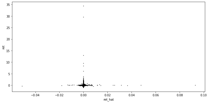
Here, after getting the result of the regression, we could use the model to predict the returns.
1
2
3
4
|
coeffient = result.params
ret_hat = debt_to_mkt_roi_table[['d2m', 'roi']] @ coeffient
prediction = pd.concat([ret_hat, debt_to_mkt_roi_table['ret']], axis=1)
prediction.columns = ['ret_hat', 'ret']
|
d2m    6.845391e-08
roi    1.401465e-05
dtype: float64
We could draw the scatter plot of return and predicted return to figure out if the prediction is reasonable. From the plot below, we could find out that the prediction is pretty decent(though the R-square is almost 0 in the model).
 1
 2
 3
 4
 5
 6
 7
 8
 9
10
11
12
13
|
# ret_hat.plot.scatter(x='ret_hat', y='ret', data=prediction);

fig = plt.figure()
ax = fig.add_subplot(111)
ax.scatter(prediction.ret_hat, prediction.ret, s=1, c='k')
# Fmin_ETH_USD = train_ETH_USD.F.min()
# Fmax_ETH_USD = train_ETH_USD.F.max()
# ax.plot((Fmin_ETH_USD, Fmax_ETH_USD), (Fmin_ETH_USD * beta_ETH_USD, Fmax_ETH_USD * beta_ETH_USD), c='r')
plt.xlabel('ret_hat')
plt.ylabel('ret')
# plt.xlim(Fmin_ETH_USD, Fmax_ETH_USD)
plt.tight_layout()
plt.show()
|
Compute the strategy.
 1
 2
 3
 4
 5
 6
 7
 8
 9
10
11
12
13
14
15
16
17
18
19
20
21
22
23
24
25
|
multi_ratio_table = coeffient['d2m'] * debt_to_market_table + coeffient['roi'] * return_on_investment_table
multi_ratio_table_temp = multi_ratio_table.T


n = round(1723 * 0.1)  # number of tickers we're gonna use in the strategy

returns_table = pd.concat([STRATEGY_DATA[tic]['px'] for tic in STRATEGY_DATA], axis=1)
returns_table.columns = STRATEGY_DATA.keys()

multi_ratio_strategy = pd.DataFrame(
    [multi_ratio_table_temp.nlargest(n, t).index.tolist() +
     multi_ratio_table_temp.nsmallest(n, t).index.tolist() for t in multi_ratio_table.index],
    index=multi_ratio_table.index).shift().dropna()

coef = np.array([1] * n + [-1] * n) / (2 * n)

multi_ratio_return = pd.Series([
    returns_table.loc[t, multi_ratio_strategy.loc[t].values] @ coef
    for t in multi_ratio_strategy.index
], index=multi_ratio_strategy.index)

plt.figure()
plt.plot(multi_ratio_return.fillna(0).cumsum())
plt.ylabel('Monthly PNL')
plt.tight_layout()
|
1
|
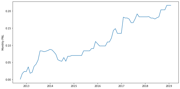
print(f'sharpe={sharpe(multi_ratio_return):.2f}, win%={win_rate(multi_ratio_return):.2%}, mdd={maximum_drawdown(multi_ratio_return):.2%}')
|
sharpe=0.10, win%=40.26%, mdd=5.80%
From the result above and the comparison between using one ratio and two ratios, we could find out that by using two ratios, the performance of the strategy is better.
3. Discussion about Sizing
The concept of sizing position by rank is that, instead of equally longing the top-10 percentile of the portoflio and equally going short the bottom-10 percentile of the portfolio, we could try to implenment the idea of “better performence, higher weight” in the strategy, which means that if the performance of the portfolio is ranked, we could give more weight to the higher ranked portfolio in order to better our performance.
Following, I tried to implement this idea into the multi-index strategy I talked before.
 1
 2
 3
 4
 5
 6
 7
 8
 9
10
11
12
13
14
15
16
17
18
19
20
21
22
23
24
25
26
27
28
29
|
multi_ratio_table = coeffient['d2m'] * debt_to_market_table + coeffient['roi'] * return_on_investment_table
multi_ratio_table_temp = multi_ratio_table.T


n = round(1723 * 0.1)  # number of tickers we're gonna use in the strategy
n -= n % 2

returns_table = pd.concat([STRATEGY_DATA[tic]['px'] for tic in STRATEGY_DATA], axis=1)
returns_table.columns = STRATEGY_DATA.keys()

multi_ratio_strategy = pd.DataFrame(
    [multi_ratio_table_temp.nlargest(n, t).index.tolist() +
     multi_ratio_table_temp.nsmallest(n, t).index.tolist() for t in multi_ratio_table.index],
    index=multi_ratio_table.index).shift().dropna()


coef = np.array(list(np.arange(n, 0, -1)) + list(np.arange(-n, 0, 1)))
coef = coef / abs(coef).sum()


multi_ratio_return = pd.Series([
    returns_table.loc[t, multi_ratio_strategy.loc[t].values] @ coef
    for t in multi_ratio_strategy.index
], index=multi_ratio_strategy.index)

plt.figure()
plt.plot(multi_ratio_return.fillna(0).cumsum())
plt.ylabel('Monthly PNL')
plt.tight_layout()
|
1
|
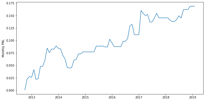
print(f'sharpe={sharpe(multi_ratio_return):.2f}, win%={win_rate(multi_ratio_return):.2%}, mdd={maximum_drawdown(multi_ratio_return):.2%}')
|
sharpe=0.08, win%=38.96%, mdd=6.39%
Not as expected, the adjusted return is actually not better than the strategy we used before. I think the intuition of this idea is reasonable, but maybe the sample size of this strategy is too small, which could not represent the overall performance of this idea. What’s more, I just used arange() to pick the position size of this strategy, I believe there’re more reasonable sizing ways to improve the performance of this idea. Also, different combination of different indexes have different performances. Those are things we could work on in the future.
4. Conclusion
In this strategy, we discussed Quantile trading using different ratios. We could find out although we’re making profits, the performance of the strategy is not that ideal. There’re several ways that may improve the performance of the strategy. Since we used monthly quantile trading, changing the frequency may be a way of improvement. However, in the real world, we should be careful because there’s no free lunch in the real market and every transaction has its costs and risks. Higher frequency may be more sensitive, but we should also consider the costs there. Also, like I said above, by finding the optimized size of different positions, we potentially could also improve the performance of our strategy.